Statistical_Learning (Mechine_Learning)

Motivation

All knowledge is, in final analysis, history.

All sciences are, in the abstract, mathematics.

All judgements are, in their rationale, statistics.

–C.Radhakrishna.Rao

Referece books

• Efron, B., & Hastie, T. (2021). Computer age statistical inference, student edition: algorithms, evidence, and data science (Vol. 6). Cambridge University Press.

• Hastie, T., Tibshirani, R., & Friedman, J. (2009). An introduction to statistical learning.

• Casella, G., & Berger, R. (2024). Statistical inference. Chapman and Hall/CRC.

• Hastie, T., Tibshirani, R., & Friedman, J. (2009). The elements of statistical learning.

statistics history

population \(f(x;\theta)\) and \(\theta\) is unknown

old/classical: Bayesian estimation; moment estimation

Moment estimation

• For the moment estimation, we do not know the density so we could not calculate the expectation directly. Instead, we use LLN to approximate the expectation with sample mean. We then have

\[ m_1(\theta) = E[X] \approx \bar{X} = \frac{1}{n} \sum_{i=1}^n X_i \]

then \[ \hat \theta = m_1^{-1}(\frac{1}{n} \sum_{i=1}^n X_i) \]

For the multiple parameter case, we could use multiple moments to estimate the parameters. (k equations to solve k unknown parameters). Here we do not know the precise distribution, so we could not calculate the moments directly. Instead, we use LLN to approximate the moments with sample moments.

Suppose \(X_1, X_2, \ldots, X_n\) are iid samples from the distribution with parameters \(f(x;\theta_1, \theta_2, \ldots, \theta_k)\) then by LLM.

We then have approximatedmoment equation:

\[ E[X^j] = m_j(\theta_1, \theta_2, \ldots, \theta_k) \approx \frac{1}{n} \sum_{i=1}^n X_i^j, j=1,2,\ldots,k \]

then we could solve the equations to get the estimators.

The solution \(\hat \theta_1, \hat \theta_2, \ldots, \hat \theta_k\) are the moment estimators of the parameters.

Bayesian estimation

\(f(x|\theta)\) is regarded as conditional density and the unknown parameter \(\theta\) is the condition. \(\theta\) is a random variable with prior distribution \(\pi(\theta)\).

\((X, \theta)\) has joint distribution \(f(x,\theta)=f(x|\theta)\pi(\theta)\)

Then we get the marginal distribution of \(X\):

\(f_X(x) = \int_{-\infty}^{+\infty} f(x|\theta)\pi(\theta)d\theta=\int_{-\infty}^{+\infty} f(x;\theta)\pi(\theta)d\theta\)

the Bayesian formula is

\[ \frac {P(A|C_i)P(C_i)}{\sum_j P(A|C_j)P(C_j)} =P(C_i|A)\]

\[ f(\theta|x)=\frac{f(x|\theta)\pi(\theta)}{f_X(x)} = \frac{f(x;\theta)\pi(\theta)}{\int_{-\infty}^{+\infty} f(x;\theta)\pi(\theta)d\theta} \]

Then above we have used Bayes theorem to get the posterior distribution of \(\theta\) given \(X=x\)

This is the updation of your belief or learning.

Bayesian statistics is unclear and ambiguous, but leaving us with no choice but to incorporate the most fundamental knowledge we have （不清不楚，不得不用）. We then update our understanding through experimental data. If it cannot be accomplished in one attempt, we iterate multiple times—eventually, we will gain a solid understanding of the parameters. The learning process is one of repeated iteration; there is no need to expect it to be completed in a single attempt.

When we do not know every knowledge about the model, we could use the prior of uniform distribution to represent our ignorance. That is, everyone is equally likely.

for \(f(x;\theta)\), we could calculate the expectation ; mode; CI

modern statistics

\(L(\theta) = E[R(\theta,X)]\)

\(\hat \theta = argmin_\theta L(\theta)\)

where \(R(\theta,X)\) is the loss function

Fisher: MLE

Fisher ambitious ： 不想依赖于贝叶斯，选prior的时候不能包含个人的任何认知，那就选客观的uniform分布 (Fisher ambitious: Not wanting to rely on Bayesian, when choosing prior, no personal cognition can be included. Then choose the objective uniform distribution)

\(\pi (\theta|x) {d\theta}= d\theta\) uniform

\(f(\theta|x_1, x_2, \ldots, x_n) = \frac{f(x_1, x_2, \ldots, x_n;\theta)\pi(\theta)}{\int f(x_1, x_2, \ldots, x_n;\theta)\pi(\theta)d\theta}\) = \(L(\theta)\)

\[ = \frac{f(x_1;\theta)f(x_2;\theta)\ldots f(x_n;\theta) }{\int f(x_1;\theta)f(x_2;\theta)\ldots f(x_n;\theta) d\theta}=L(\theta) \]

Mode:

Find maximum of \(f(\theta|x_1, x_2, \ldots, x_n)\) i.e. L(\(\theta\))

\(\hat \theta = argmax_\theta L(\theta)=argmax_\theta \frac{f(x_1;\theta)f(x_2;\theta)\ldots f(x_n;\theta)}{f_X(x_1,x_2,..x_n)}\)

\(= argmax_\theta f(x_1;\theta)f(x_2;\theta)\ldots f(x_n;\theta)=argmax_\theta L(\theta)\) this is the likelihood function

When Fisher wanted to publish his idea to the Royal Society, he had been harshly commented through the discussion of the Royal Society. This is a good tradition but nowadays’ conference does ntot keep this. This means now they just have a presentation but the comments will not appear in the published paper.

then we could use log likelihood to simplify the calculation of the derivative to get the maximum likelihood estimator.

modern: Loss function

Modern Statistics

Loss function is a “scanning apparatus”. It will take special value at the true parameter such as 0 or minimum point.

Empirical Kullback-Leibler Divergence Loss and MLE

(Empirical loss means that since we do not know the true distribution, we could use the sample to approximate the loss function. )

Consider the empirical loss function：

\[l(\theta) = \mathbb{E}_{\Theta} \left[ \frac{f(x;\theta_0)}{f(x;\theta)} \log \frac{f(x;\theta_0)}{f(x;\theta)} \right]\]

\[= \int \frac{f(x;\theta_0)}{f(x;\theta)} \log \frac{f(x;\theta_0)}{f(x;\theta)} f(x;\theta) dx\]

\[= \int \left[ \log \frac{f(x;\theta_0)}{f(x;\theta)} \right] f(x;\theta_0) dx\]

\[= \mathbb{E}_{\Theta_0} \left[ \log \frac{f(x;\theta_0)}{f(x;\theta)} \right]\]

\[\approx \frac{1}{n} \sum_{i=1}^{n} \log \frac{f(x_i;\theta_0)}{f(x_i;\theta)}\]

\[= \frac{1}{n} \sum_{i=1}^{n} \log f(x_i;\theta_0) - \frac{1}{n} \sum_{i=1}^{n} \log f(x_i;\theta)\]

\[\text{Argmin}(\hat{\theta}) = \text{Argmin}\left[ -\frac{1}{n} \sum_{i=1}^{n} \log f(x_i;\theta) \right]\]

\[= \text{Argmax}\left[ \sum_{i=1}^{n} \log f(x_i;\theta) \right]\]

\[= \text{Argmax}\left[ \log \prod_{i=1}^{n} f(x_i;\theta) \right]\]

KL-divergence Property

Let \(E_{\theta}\) be the expectation of \(f_{\theta}(x)\).

the true model \(f(x;\theta_0)\)，and the proposed model is \(f(x,\theta)\)。

KL (entropy) divergence:

\[\mathbb{E}_{\theta} \left[ \frac{f(x;\theta_0)}{f(x;\theta)} \log \frac{f(x;\theta_0)}{f(x;\theta)} \right]\]

Let \(\varphi(x) = x \log x\)，then \(\varphi'(x) = \log x + 1\)，\(\varphi''(x) = \frac{1}{x} > 0\)，

So \(\varphi(x)\) is a convex function over \((0,+\infty)\).。

By Jensen inequality：

\[\varphi\left( \mathbb{E}_{\theta} \left[ \frac{f(x;\theta_0)}{f(x;\theta)} \right] \right) \leq \mathbb{E}_{\theta} \left[ \varphi\left( \frac{f(x;\theta_0)}{f(x;\theta)} \right) \right]\]

\[\mathbb{E}_{\theta} \left[ \frac{f(x;\theta_0)}{f(x;\theta)} \right] = \int_{-\infty}^{\infty} \frac{f(x;\theta_0)}{f(x;\theta)} f(x;\theta) dx\]

\[= \int_{-\infty}^{\infty} f(x;\theta_0) dx = 1\]

Thus

\[\varphi(1) = 1 \times \log 1 = 0 \leq \mathbb{E}_{\theta} \left[ \frac{f(x;\theta_0)}{f(x;\theta)} \log \frac{f(x;\theta_0)}{f(x;\theta)} \right]\]

Loss function

\[l(\theta) = \mathbb{E}_{\theta} \left[ \frac{f(x;\theta_0)}{f(x;\theta)} \log \frac{f(x;\theta_0)}{f(x;\theta)} \right] \geq 0\]

and \(l(\theta_0) = 0\)，so \(\theta_0\) is \(l(\theta)\)’s minimum point

Empirical estimators are:

\[l(\theta) \approx \frac{1}{n} \sum_{i=1}^n \frac{f(x_i;\theta_0)}{f(x_i;\theta)} \log \frac{f(x_i;\theta_0)}{f(x_i;\theta)}\]

Conclusion: Maximum likelihood estimation is equivalent to minimizing the KL divergence, which provides the theoretical basis of information theory for MLE.

Remark: differences between divergence and distance

• Divergence is different from the distance since

  • d(a,b) \(\neq\) d(b,a).

  • it does not satisfy the triangle inequality

For example, \(a/b\) is not the distance but a kind of divergency

DeepSeek loss function—Feed the data - gradient descent—LLM

Sufficient statistics

\[ \hat \theta =T(X_1, X_2, \ldots, X_n) \] where

\[ T : R^n \to R \] The sufficient statistics is a compression of the data that retains all the information needed to estimate the parameter \(\theta\); It is the filtering of the information that thorwing away the noise; It is the distillation of the data that keeps the essence. Therefore, the sufficiency means no information is lost and we combine the information into 2 numbers.

• Two sufficient statistics have invertible transformation between them. Therefore there are many sufficient statistics.

• sufficient statistics is not unbiased

Rao-Blackwell Theorem

• Motivation: not only do we need the sufficiency of the statistics, but also we want the estimator to be unbiased and with minimum variance.

• the proof includes the idea of changing the double expectation into the iterated expectation with one of it to be the conditional expectation(just like changing the double integral into the iterated integral). This proof demonstrates the charisma of the conditional expectation which improves the efficiency.

Sampling distribution

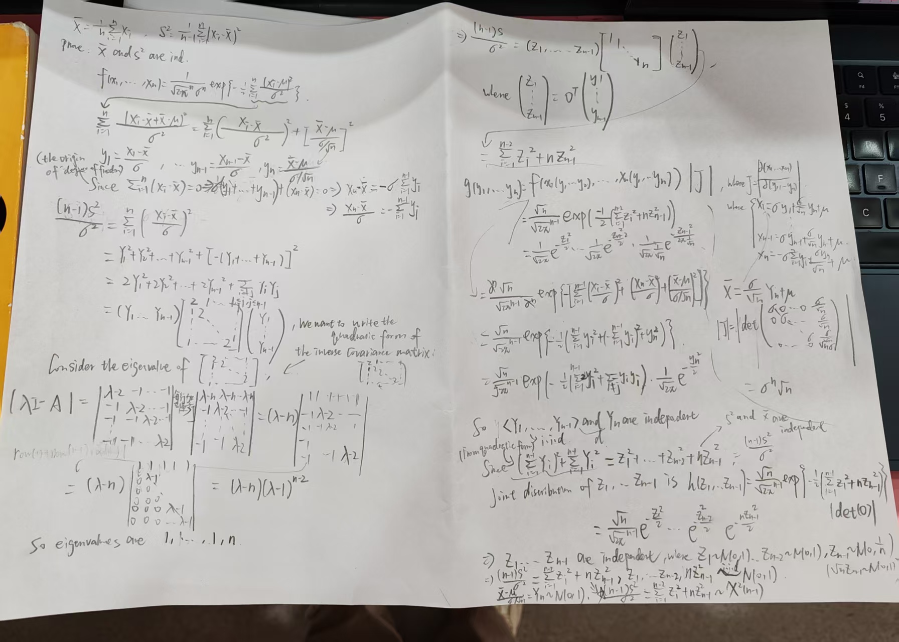
the proof of the independence of the sample mean and sample variance

gitgit

Linear Regression

OLS

\((y-Xw)^T \Sigma ^{-1 }(y-Xw)\)

homo assumption: \(\Sigma = \sigma^2 I\) (a circle) but this can also be generalized to \(\Sigma = \sigma^2 D\) where \(D\) is a diagonal matrix (a ellipse).

\(X(X^TX)^{-1}X^T\) could be seen as a projection matrix, so if \(w=(X^TX)^{-1}X^Ty\), then \(Xw\) is the projection of \(y\) onto the column space of \(X\). From a similar perspective, \(y-Xw\) is the residual vector, which is orthogonal to the column space of \(X\).

If singular, use psuedo-inverse: \(w = X^+y\) that could be linked to SVD, where \(X^+\) is the Moore-Penrose pseudo-inverse of \(X\), where SVD is \(X = U \Sigma V^T\), then \(X^+ = V \Sigma^{-1} U^T\). –this case has many solutions.

Remark: often we have n >> d+1, so the matrix \(X^TX\) is invertible, but if \(n < d+1\), then \(X^TX\) is singular, and we need to use the pseudo-inverse. (\(X^TX\) is invertible if and only if the columns of \(X\) are linearly independent, which is often the case in practice when n >> d+1 , but not always.)

Eg Simplified Ceres Orbit Problem

SEE PPT

Gauss’s secret Weapon —- observe 3 points

200 years ago: agrues about the relationship of the linear regression and Normal — think of MLE

regularization

It is used to limited the situation that n < d+1

loss function

Why using square : —- firstly, the geometric meaning — projection

MLE

Likelihood function

Asymptotic property

Consistency

Assumptions:

Asympotic Normalty

Asymptotic unbiasedness (although not unbiased)

NEED TO ADD 3 cases of the Cramer-Rao Lower bound

• general

• • i.i.d assumption

\[ \text{var}_\theta \left( \hat{\gamma}_n \right) \geq B_n(\theta) \equiv \frac{\left[ \frac{dE_\theta(\hat{\gamma}_n)}{d\theta} \right]^2}{nI(\theta)} \]

Remark.(interpretation of the information matrix’s intuitive meaning in this Thm In this corollary,\(f(x, \theta)\) is the PMF/PDF of each random variable\(X_i\), while\(f_{X_n}(x_n, \theta)\) in the previous theorem is the joint PMF/PDF of the random sample\(X_n\). Under the IID assumption, it is clear that the Cramer-Rao lower bound\(B_n(\theta)\) vanishes to zero at a rate\(n\).

In addition to the scale factor\(n^{-1}\), the Cramer-Rao lower bound is proportional to the inverse of Fisher’s information matrix\(I(\theta)\). Fisher’s information matrix\(I(\theta)\) measures the degree of information about\(\theta\) that is contained in the population PMF/PDF\(f(x, \theta)\) or equivalently in each random variable\(X_i\). The larger\(I(\theta)\), the more information about\(\theta\) is contained in the random variable\(X_i\). As a consequence, we have a smaller\(B_n(\theta)\).

Remark. The calculation of \(I(\theta)\) sometimes is tedious. By using the information matrix equality \(I(\theta) + H(\theta) = 0\), where

\[ H(\theta) \equiv E_\theta \left[ \frac{\partial^2 \ln f(X_i, \theta)}{\partial \theta^2} \right] = \int_{-\infty}^{\infty} \frac{\partial^2 \ln f(x, \theta)}{\partial \theta^2} f(x, \theta) dx \]

is called the Hessian matrix, we can write the Cramer-Rao lower bound

\[ B_n(\theta) = \frac{[E_{\theta}'(\hat\tau(\theta))]^2}{-nH(\theta)} \]

Thus, the Cramer-Rao lower bound \(B_n(\theta)\) depends on the inverse of the curvature of the log-likelihood function \(\ln f(x, \theta)\). The larger the curvature in absolute value, the smaller the Cramer-Rao lower bound \(B_n(\theta)\).

• • (asymptotic) unbiasedness assumption

\[ B_n(\theta) = \frac{[\tau'(\theta)]^2}{-nH(\theta)} \]

• In particular, for MLE

We have shown that the MLE

\[ \sqrt{n} \left( \hat{\theta}_n - \theta_0 \right) \xrightarrow{d} N \left[ 0, -H(\theta_0)^{-1} \right] \text{ as } n \rightarrow \infty, \]

Besides,

Let the \(\hat \gamma_n\) be an estimator of \(\theta\) which is unbiased asymptotically.

\[ d \theta/d \theta=1 \]

We concludes that this reaches the cramer lower bound.

This implies \(\hat{\theta}_n - \theta_0\) approximately follows a \(N \left\{ 0, [ -nH(\theta_0)]^{-1} \right\}\) for \(n\) sufficiently large. Thus, the variance of the MLE \(\hat{\theta}_n\) approximately achieves the Cramer-Rao lower bound when \(n\) is large. This is true for any population distribution \(f(x, \theta_0)\). Given the asymptotic normality of \(\sqrt{n} \left( \hat{\theta}_n - \theta_0 \right)\), the asymptotic bias of the MLE \(\hat{\theta}_n\) is zero. It follows that MLE \(\hat{\theta}_n\) is asymptotically most efficient.

MLE’s asymptotic normality + Cramer-Rao Lower bound obtains that MLE is the most efficient for all asymptotic unbiased estimators!!

Eg

For the simple linear regression,

since

\[ \sqrt n (\hat \beta_{MLE}-\beta) \rightarrow^d N(0,I^{-1}) \]

Avar(Asymptotic variance) \(\sqrt n \hat \beta_{MLE}\)=Avar\(\sqrt n(\hat \beta_{MLE}-\beta)\) =\(I ^{-1}\)

Let Avar (\(\sqrt n \hat \beta_{OLS}\)) =B

Since Cramer-Rao Lower bound tells us that over a class of estimators,we have a theoretical minimum level (if the estimator is unbiased for i.i.d. samples, this is actually \(I^{-1}\) ) of the (asymptotic) variance for these estimators, we always have

\[ I^{-1} - B \text{ is non-positive definite} \] i.e.

$$ v, v^T(I{-1} - B)v

$$

Therefore, we could interpret the BLUE of OLS using the Asymptotic unbiasedness of MLE, also. Since the estimators derived by OLS and ML are the same. However, if the residual does not assumed to be normal then the MLE is more efficient than OLS. Alough this is the case, please bear in mind that there is always a cost when using MLE—Once the assumption of the distribution is not suitable or too inflexible, it is even better to choose OLS.

Remark: Uniform distribution is better to be estimated using moment estimator since \(\theta\) is not an interior point of its parameter space

See notes P145

ps: parameter statistics

Suppose the data satisfies the normal distribution — in that case, we could use the mean = \(\mu = \frac{1}{n} \sum_{i=1}^n x_i\)

skew

mean > median > mode — right skew

skew should use median or mode to represent some characteristic

Gaussion did not publish until 9 years later, he has really understood the relationship between linear regression and normal distribution,

WLS

Standard OLS assumes Var(εi ) = σ2 (constant variance)

Real-world data often violate this assumption, leading to heteroscedasticity (non-constant variance of errors), say Var(εi ) = σ2 Di or = \(\sigma_i^2\), where Di is a diagonal matrix with varying variances for each observation.

OLS estimates remain unbiased but not efficient (higher variance than necessary) when the errors are heteroscedastic (i.e., the variance of the errors is not constant across observations).

( error satisfies the normal distribution” fix x and we hace the points follow normal distribution)

Consequences of ignoring the heteroscedasticity:

\((y-Xw)^T \Sigma ^{-1 }(y-Xw)\)

\(\Sigma ^{-1 }\) is the weight matrix which is diagonal for uncorrelated errors and could be a full matrix for correlated errors.

Remark: standard OLS assumes \(\Sigma = \sigma^2 I\), which is a special case of the weighted least squares where all weights are equal.

Problem: can not know D, So we use the weighted least squares to estimate D (iteration)

Now, the weighted residual sum of squares is:

\[ (y-Xw)^T \Sigma^{-1} (y-Xw) \]

Let $ D = ^{-1} $, then the weighted residual sum of squares is:

\[ y^TDy - 2w^TX^TDy + w^TX^TDXw \]

\(\hat w_{OLS} = (X^TDX)^{-1}X^TDy\)

import statsmodels.api as sm
mod_wls = sm.WLS(y, X, weights=1/var_est)
res_wls = mod_wls.fit()

Concave and Hessian Matrices

(Semi-) Defined Matrices

For the non-eigenvector x, the role of matrix A can be regarded as projecting x onto the eigenvector basis and then stretching it in each basis direction.

Since the eigenvalues are non-negative, this stretching will not reverse the direction of the vector in any direction. From the perspective that the space of A is A linear combination of its eigenvector and generalized eigenvector, explain why the role of matrix A can be regarded as projecting x onto the basis of the eigenvectors:

Under the basis of the eigenvectors, when we apply A to a vector x, we can think of it as first projecting x onto the subspace spanned by the eigenvectors (write x as the linear combination of eigenvectors) and then stretching it according to the eigenvalues associated with those eigenvectors (Ax=\(\lambda\)x).

• Remark: We do not need to consider the generalized eigenvectors here. This is because whether it is a positive definite, semi-positive definite or negative definite matrix, their eigenvectors can support the entire space without the need for generalized eigenvectors. This is because these matrices are all symmetric matrices, and symmetric matrices can always be diagonalized, and their eigenvectors can form a set of bases in space, i.e.

Since \[ A = A ^T \] and \[ Av_1 = \lambda_1 v_1 \] and \[ Av_2 = \lambda_2 v_2 \]

then we have

\[ v_2^TAv_1=\lambda_1 v_2^Tv_1 \] Since \(A=A^T\),

\[ v_2^TAv_1 = (Av_2)^Tv_1 = \lambda_2 v_2^Tv_1 \]

So

\[ \lambda_1 v_2^Tv_1 = \lambda_2 v_2^Tv_1 \]

So

if \(\lambda_1 \neq \lambda_2\), then \(v_2^Tv_1 = 0\), which means \(v_1\) and \(v_2\) are orthogonal and therefore can form a basis of the space.

??? USe the understanding of “Left multiplication” to explain why the role of matrix A can be regarded as projecting x onto the basis of the eigenvectors:

if X has full rank, then \(X^TX\) is positive definite.

• Singular Value Decomposition (SVD):

Every matrix can be decomposed into the product of three matrices: \(X = U \Sigma V^T\), where \(U\) and \(V\) are orthogonal matrices and \(\Sigma\) is a diagonal matrix with non-negative entries (the singular values). The columns of \(U\) and \(V\) are the left and right singular vectors, respectively.

We now have:

\[ X^TX= V \Sigma^T U^T U \Sigma V^T = V \Sigma^2 V^T \]

This means that the eigenvalues of \(X^TX\) are the squares of the singular values of \(X\), which are non-negative. Therefore, \(X^TX\) is positive semi-definite.

When X has full rank, all singular values are positive, and thus \(X^TX\) is positive definite.

\(X^TAX\) is a elliptic

\(A=Q\Lambda Q^T\) is the eigendecomposition of \(A\), where \(Q\) is an orthogonal matrix whose columns are the eigenvectors of \(A\), and \(\Lambda\) is a diagonal matrix whose diagonal entries are the eigenvalues of \(A\).

Then we have:

\[ X^TAX = X^TQ\Lambda Q^TX = (Q^TX)^T\Lambda (Q^TX) = Y^T\Lambda Y=1 \]

where \(Y = Q^TX\).

this is saying \(\lambda_1 y_1^2 + \lambda_2 y_2^2 + ... + \lambda_n y_n^2 = 1\), where \(lambda_i\) are the eigenvalues of \(A\) and \(y_i\) are the components of the vector \(Y\).

If \(\lambda_i > 0\) for all \(i\), then this is an equation of an ellipsoid in the space spanned by the eigenvectors of \(A\). A special case is when all \(\lambda_i\) are equal, which corresponds to a sphere or a circle in 2D.

See 3 blue 1 brown video

Mahalanobis distance and Euclidean distance

The differences between the Euclidean distance and Mahalanobis is the linear transformation

Categorical variables in linear / logistic regression –reference variable

glm

• random component: \(p (y|\theta, \phi) = exp ( (y \theta - b(\theta)) / a(\phi) + c(y, \phi) )\)

• systematic component: \(Xw\)

• link function:

special case : logistic regression

软分类 给概率而非分到哪一类

Supervised learning: 既定事实—-0，1

unsupervised learning： 无既定事实

机器学习： 感知机 （单个神经元）

非线形： 线性套函数

why logit

from 1 to 0 ;

KL distance — whethere the 2 distributions have significant difference

xiangnong 香浓shang

no analytic solution – Newton-Raphson method (IRLS) / gradient Ascent – only suitable for concave function

\(w^{(t+1)} = w^{(t)} + \lambda ..\), where the lambda is called the rate of learning – too small might be slow, too large might be in a cycle which could not be converge

training data and test data

2,8 分 — cross validation

• Extension of logistic regression : Softmax regression (multinomial logistic regression) – multiple classes

Micro jordan

Cross-entropy loss

neural networks use it

batch effect

可解释性神经网络： 给理由为什么lambda

alphago： 不懂围棋的人用足够厉害的算法就能赢

x \(->^f\) x — score to decide the goodness of f

Fisher’s discriminant analysis (FDA) – linear discriminant analysis (LDA) – linear regression

Contribution:

Perceptron algorithm

LDA has the analytic solution

激活函数

logistic

RELU

Perceptron

Logistic regression

Surf poster– gradient accent

variable transformation formula–the first conversation with Dr. Zhu

• idea: CDF’s derivative is PDF and ..

Assume we have two random variables \(X\) and \(Y\), where \(Y = g(X)\) is a monotonic and differentiable function of \(X\). Our goal is to find the probability density function \(f_Y(y)\) of \(Y\), given the probability density function \(f_X(x)\) of \(X\).

Variable Transformation Formula

The variable transformation formula is stated as follows: \[f_Y(y) = f_X(g^{-1}(y)) \left| \frac{d}{dy} g^{-1}(y) \right|\]

Proof Process

1. Transformation of the Cumulative Distribution Function (CDF):

   First, consider the cumulative distribution function \(F_Y(y)\) of \(Y\), which is defined as the probability that \(Y\) is less than or equal to \(y\):

   \[F_Y(y) = P(Y \leq y)\] Since \(Y = g(X)\), we can express this probability in terms of \(X\):

   \[F_Y(y) = P(g(X) \leq y)\]

2. Using the Inverse Function Transformation:

   If \(g(x)\) is strictly increasing (or strictly decreasing), then \(g(X) \leq y\) is equivalent to \(X \leq g^{-1}(y)\) (or \(X \geq g^{-1}(y)\)). Therefore:

   \[F_Y(y) = P(X \leq g^{-1}(y)) = F_X(g^{-1}(y))\]

   where \(F_X(x)\) is the cumulative distribution function of \(X\).

3. Deriving the Probability Density Function (PDF):

   To find the probability density function \(f_Y(y)\) of \(Y\), we need to differentiate \(F_Y(y)\) with respect to \(y\):

   \[f_Y(y) = \frac{d}{dy} F_Y(y) = \frac{d}{dy} F_X(g^{-1}(y))\]

   Using the chain rule, we get:

   \[f_Y(y) = f_X(g^{-1}(y)) \frac{d}{dy} g^{-1}(y)\]

4. Considering the Absolute Value of the Derivative:

   Since the probability density function must be non-negative, we take the absolute value of the derivative: \[f_Y(y) = f_X(g^{-1}(y)) \left| \frac{d}{dy} g^{-1}(y) \right|\]

This completes the proof of the variable transformation formula. This formula is very useful when dealing with transformations of random variables, especially in statistical analysis and probability modeling. With this formula, we can derive the probability density function of one related random variable from the known probability density function of another.

Sampling Methods

Bootstrap

Example of calculating p-value of KS-statstics (Goodness of fit) with the problem of censoring data distribution estimate

Research Question: No Difference Between Empirical (KM-method) and Theoretical Distributions(estimated) (Does My Interval-Censored Data Come from the Estimated (theoretical) Distribution?)

Null Hypothesis: The data indeed come from the estimated distribution.

Steps of the Parametric Bootstrap Method:

1. Simulate a World Where the Null Hypothesis Holds:

   • Generate a large number (B = 1000) of new samples from the estimated distribution.

   • Apply the exact same interval-censoring structure to each new sample (using the original left_times and right_times).

   Assume the observed time points does not change

2. Calculate Bootstrap KS Values:

   • For each bootstrap sample, compute the KS-statistic.

   • Obtain 1000 bootstrap KS values (ks_bootstrap).

3. Calculate the p-value:

   • p = (number of ks_bootstrap \(≥\) ks_stat) / B (a larger ks-stat indicates a greater difference between the data and the distribution).

Interpretation: - A large p-value: If H₀ is true, the probability of observing a KS statistic as large as that from the original data is high. Therefore, we do not have sufficient evidence to reject H₀ and conclude that the data likely come from this estimated distribution. This is because a large p-value implies that it is quite probable to generate a sample with a difference from the theoretical distribution at least as large as that observed in the current data. In other words, the observed difference is not unusual and falls within the normal range of random variation. Hence, we cannot reject the hypothesis that the data come from the estimated distribution.

Some Perspectives to Penalized Regression Mode

OLS / MLE Solution to LR with issues

We have learned the equivalence of Ordinary Least Squares (OLS) and Maximum Likelihood Estimation (MLE) in the context of linear regression assuming the error term follows a Gaussian distribution but with limitations as below:

• Issues:

Even if the OLS or MLE solution is optimal in terms of minimizing the error, it may lead to overfitting, especially when the number of features is large relative to the number of observations. This can result in high variance and poor generalization to new data.

How to handle the issues?

\[\begin{align*} \text{LASSO:} & \quad Argmin_{\beta} \sum_{i=1}^{N} \left( y_i - \sum_{j}^{p} \beta_j x_{ij} \right)^2 + \lambda \sum_{j}^{p} |\beta_j|, \quad \text{where } \lambda > 0 \\ \text{Ridge:} & \quad Argmin_{\beta} \sum_{i=1}^{N} \left( y_i - \sum_{j}^{p} \beta_j x_{ij} \right)^2 + \lambda \sum_{j}^{p} \beta_j^2, \quad \text{where } \lambda > 0 \end{align*}\]

• OLS perspective thinking: This shrinkage method not only achieves the objective of making the error to be smallest like OLS, but also prevents overfitting by penalizing large coefficients.

• MLE perspective thinking: Compared with MLE, this method could be regarded as a Bayesian estimation that can avoid overfitting by introducing the prior distribution \(P(\beta)\), especially when the data volume is small, the prior information can play a regularization role.

Why does the terms of the regularization look like this?

Just like what we have learned about the relationship between the OLS and MLE and get the idea of why the error term is the square shape, now we are going to use the perspective of Bayesian to understand the penalized terms

Choose Prior Distribution \(P(\beta)\)

Idea:

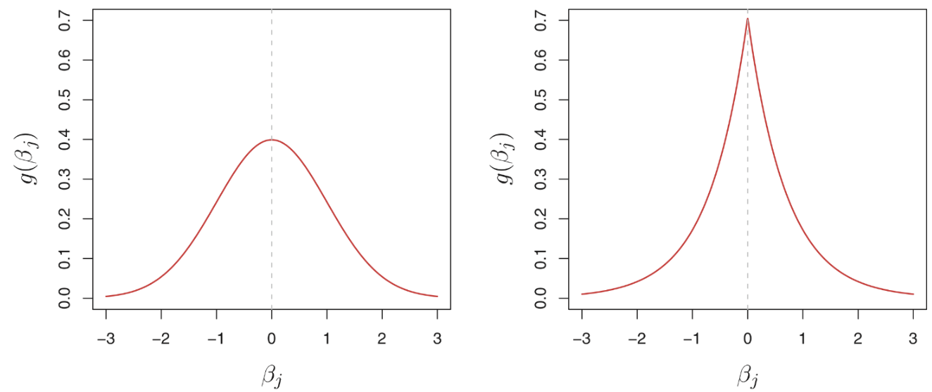
We insist that \(\beta\) should be more likely to be small also with small variances (very near to 0). This means we should pick a distribution that has a peak around zero and decays quickly as we move away from zero.

• Prior Distribution: In the context of penalized regression, we choose a prior distribution for the coefficients \(\beta\) that reflects our beliefs about their values. Common choices include:
  • Laplace Prior: Assumes coefficients follow a Laplace distribution, leading to \(L^1\) regularization (Lasso Regression).
  • Gaussian Prior: Assumes coefficients are normally distributed around zero, which leads to \(L^2\) regularization (Ridge Regression).

This also means it would take extreame evidence with the data that we see in order to accept very large and very high variances beta because of the prior.

Choose Prior Distribution \(P(\beta)\)

Maximize the posterior probability to get the point estimation of \(\beta\) – Ridge

\[ P(\beta|y) \propto P(y|\beta) \cdot P(\beta) \]

\[ P(y|\beta) = \frac{1}{\sqrt{2\pi}\sigma} \exp\left\{-\frac{(y - \beta^T x)^2}{2\sigma^2}\right\} \]

And for the prior part, we assume \(beta\) follows a Gaussian distribution, $(0, ’^2) $,

\[ P(\beta) = \frac{1}{\sqrt{2\pi}\sigma'} \exp\left\{-\frac{\beta^2}{2\sigma'^2}\right\} \]

Thus,

\[ \hat{\beta} = \arg\max_\beta \log P(\beta|Y) \]

\[ = \arg\max_{\beta} \log P(Y|\beta)P(\beta) \]

\[ = \arg\max_{\beta} \log \prod_{i=1}^N P(y_i|\beta)P(\beta) \]

\[ = \arg\max_{\beta} \sum_{i=1}^N \log[P(y_i|\beta)P(\beta)] \]

\[ = \arg\max_{\beta} \sum_{i=1}^N \left[ \log\left(\frac{1}{\sqrt{2\pi}\sigma } \exp\left\{-\frac{(y - \beta^T x)^2}{2\sigma^2}\right\}\right) + \log(\frac{1}{\sqrt{2\pi}\sigma'})- \frac{\beta^2}{2\sigma'^2} \right] \]

\[ = \arg\max_{\beta} \sum_{i=1}^N \left[ \log\left(\frac{1}{2\pi \sigma' \sigma}\right) - \frac{(y_i - \beta^T x_i)^2}{2\sigma^2} - \frac{\beta^2}{2\sigma'^2} \right] \]

\[ = \arg\min_\beta \sum_{i=1}^N \left[ \frac{(y_i - \beta^T x_i)^2}{2\sigma^2} + \frac{\beta^2}{2\sigma'^2} \right] \]

\[ = \arg\min_\beta (Y-X\beta)^T (\frac{1}{2\sigma^2}I_N) (Y-X\beta) + \frac{1}{\sigma'^2} \beta^2 \]

((Weighted least squares with the weight \(\frac{1}{2\sigma^2}I_N\) and the penalty term \(\frac{1}{\sigma'^2} \beta^2\)

If we let \(\lambda = \frac{1}{\sigma'^2}\), then the loss function is \(L(\beta) = \sum_{i=1}^N (\beta^T x_i - y_i)^2 + \lambda \beta^T \beta\), which is equivalent to the minimization of the regularized least squares in \(L^2\).

• Remark of the Ridge Regression

Ridge regression solution is also the posterior mean, this is because the likelihood of the data given the parameters is Gaussian, and the prior is also Gaussian, which results in a posterior that is also Gaussian by the property of the conjugate prior of the Gaussian distribution, i.e.

NEED to ADD!

Maximize the posterior probability to get the point estimation of \(\beta\) – Lasso

Now the prior part is assumed to be a Laplace distribution, \(\beta \sim \text{Laplace}(0, b), i.e., P(\beta) = \frac{1}{2b} \exp\left(-\frac{|\beta|}{b}\right)\).

\[ \arg\max_{\beta} \sum_{i=1}^N \left[ \log\left(\frac{1}{\sqrt{2\pi}\sigma_{\beta} } \exp\left\{-\frac{(y - \beta^T x)^2}{2\sigma^2}\right\}\right) - \log 2b - \frac{|\beta|}{b} \right] \]

\[ = \arg\max_{\beta} \sum_{i=1}^N \left[ \log\left(\frac{1}{\sqrt{2\pi}\sigma_{\beta} 2b}\right) - \frac{(y_i - \beta^T x_i)^2}{2\sigma^2} - \frac{|\beta|}{b} \right] \]

\[ = \arg\min_\beta \sum_{i=1}^N \left[ \frac{(y_i - \beta^T x_i)^2}{2\sigma^2} + \frac{|\beta|}{b} \right] \]

\[ = \arg\min_\beta (Y-X\beta)^T (\frac{1}{2\sigma^2}I_N) (Y-X\beta) + \frac{1}{b} |\beta| \]

If we let \(\lambda = \frac{1}{b}\), then the loss function is \(L(\beta) = \sum_{i=1}^N (\beta^T x_i - y_i)^2 + \lambda |\beta|\), which is equivalent to the minimization of the regularized least squares in \(L^1\).

Further check \(\lambda\) and corresponding term in the posterior likelihood–How the penalized terms are derived from the Bayesian perspective

Gaussian:

\(\lambda = \frac{1}{\sigma'^2}\) i.e. Larger \(\lambda\) with less \(\sigma'^2\) means more regularization corresponding to smaller variance of the prior distribution (normal)

Laplace:

\(\lambda = \frac{1}{b}\) i.e. Larger \(\lambda\) with less \(b\) means more regularization corresponding to smaller variance of the prior distribution (laplace)

How to choose the \(\lambda\)?

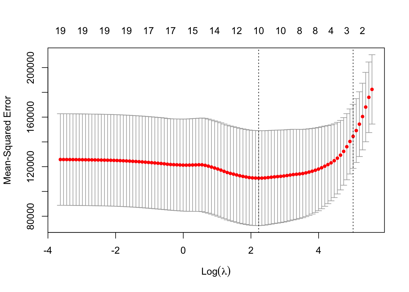
• Cross-Validation: A common method to choose the regularization parameter \(\lambda\) is through cross-validation. This involves splitting the data into training and validation sets, fitting the model with different values of \(\lambda\), and selecting the one that minimizes the prediction error on the validation set.

Lagrange Multipliers Perspective of Penalized Models

Lagrange multipliers provide a way to incorporate constraints into optimization problems. In the context of penalized regression, we can view the regularization term as a constraint on the size of the coefficients.

Choose Lasoo as an example, the Lagrange multipliers perspective could be expressed as:

\[ \left( \hat{\alpha}, \hat{\beta} \right) = \arg \min \left\{ \sum_{i=1}^{N} \left( y_{i} - \alpha - \sum_{j} \beta_{j} x_{ij} \right)^{2} \right\} \quad \text{subject to} \quad \sum_{j} \left| \beta_{j} \right| \leq t. \]

i.e.

\[ g(\beta)= \sum_{j} \left| \beta_{j} \right| - t \leq 0 \]

\[ L(\alpha,\beta, \lambda) = \sum_{i=1}^{N} \left( y_{i} - \alpha - \sum_{j} \beta_{j} x_{ij} \right)^{2} + \lambda \left( \sum_{j} \left| \beta_{j} \right| - t \right) \]

\[ \partial L / \partial \alpha = 0 \]

\[ \hat{\alpha} = \bar{y} - \sum_{j} \hat{\beta}_{j} \bar{x}_{j} \]

\[ \partial L / \partial \beta_{j} = 0 \]

\[ -2 \sum_{i=1}^{N} x_{ij} \left( y_{i} - \hat{\alpha} - \sum_{k} \hat{\beta}_{k} x_{ik} \right) + \lambda \cdot sign(\hat{\beta}_{j}) = 0 \]

This may use the iterative method to solve the equation.

Generally, the formula could be expressed as:

\[ \min_{\beta} \left\{ \lVert y - X\beta \rVert_2^2 + \lambda \lVert \beta \rVert_p^p \right\} \]

where \(\lVert \beta \rVert_p^p\) is the \(L^p\) norm of the coefficients, which serves as a penalty term.

The gradient of the objective function of Ridge with respect to \(\beta\) is given by:

\[ \nabla J(\beta) = -2X^T(y - X\beta) + \lambda \nabla \lVert \beta \rVert_p^p \]

(see matrix form (Go to Matrix Form) below for more details)

This should be set to zero to find the optimal \(\beta\), which means the gradient of the loss function (the first term) is equal to the gradient of the penalty term (the second term) scaled by \(\lambda\).

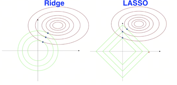
Geometric Interpretation of Penalized Models in Lagrange Multipliers Perspective

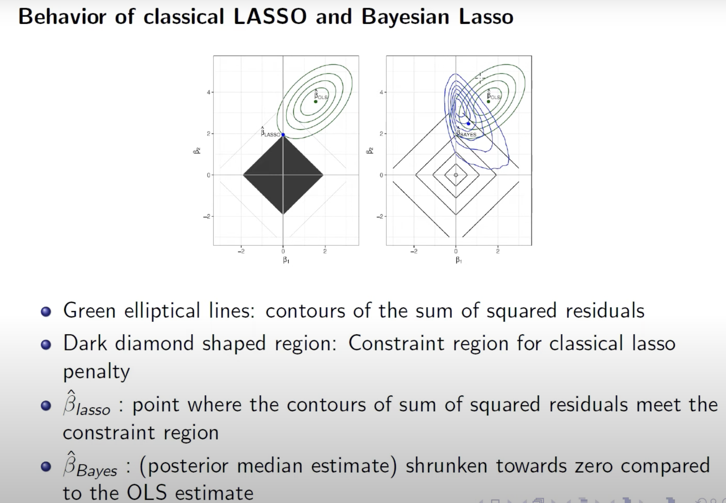
Geometric Interpretation of LASSO in Lagrange Multipliers Perspective and Bayesian Perspective

Story

• Humorous story

Ryan Tibshirani interviews Rob Tibshirani about his work on the Lasso. Ryan said that when he was young he was into draw a diamond and circles and he happened to draw a circle that just touched the corner of a diamond and that led to a big idea Rob did not credited him for. “I did not cite you,” Rob answered humorously.

• Idea

Yes, this is actually an interesting geometric meaning of LASSO.

• To me(a biostat student) —a big meaning!!

Rob Tibshirani previously went back to his hometown of Toronto when he was a professor in preventative medicine and biostatistics and he was working on LASSO here.

Story—Rob Tibshirani’s motivation

• Paper about non-negative garrote by Leo Breiman

  Leo started with least squares estimates and then multiply them by non-negative constants that were bounderd by some bounded T, which had the effect of producing a sparse solution because being non-negative with a bound of 0 forces sparsity.

• why choose “Lasso” name

  More gentle than garrote and more softer term than garrote

• Many similar things that time

  You do not need to do research on unique things, but promising things.

• From LM to GLM to Cox, this generalization is cool

Understanding of \(\lambda\)

Lagrange Multipliers help explain how \(\lambda\) balances fitting the data well:

Bigger \(\lambda\) makes the ellipse (representing the constraint region in the parameter space in WLS, if it satisfies the homoscedasticity, it would be a circle) smaller. In this case, the gradient of \(\beta\) becomes steeper with a larger \(\lambda\), which means that the optimization algorithm will grow the penalty of \(\beta\) to stay within the shrinking feasible region. This helps reduce variance and prevent overfitting, but overly large \(\lambda\) can cause underfitting.

Matrix Form of Penalized Regression Models

Ridge Regression

Objective Function

\[ \min_{\beta} \left\{ \lVert y - X\beta \rVert_2^2 + \lambda \lVert \beta \rVert_2^2 \right\} \]

Matrix Form Derivation:

• Expand the loss term: \[ \lVert y - X\beta \rVert_2^2 = (y - X\beta)^T (y - X\beta) = y^T y - 2y^T X\beta + \beta^T X^T X\beta. \]
• Add the \(L^2\) penalty: \[ J(\beta) = y^T y - 2y^T X\beta + \beta^T X^T X\beta + \lambda \beta^T \beta. \]
• Compute the gradient: \[ \frac{\partial J}{\partial \beta} = \nabla J(\beta) = -2X^T(y - X\beta) + \lambda \nabla \lVert \beta \rVert_p^p=-2X^T y + 2X^T X\beta + 2\lambda \beta. \]
• Set gradient to zero: \[ -X^T y + X^T X\beta + \lambda \beta = 0 \implies (X^T X + \lambda I)\beta = X^T y. \]
• Solve for \(\beta\): \[ \hat{\beta}_{\text{ridge}} = (X^T X + \lambda I)^{-1} X^T y \]

Why Regularization Helps:

The term \(\lambda I\) ensures \(X^T X + \lambda I\) is always invertible (since \(\lambda > 0\) adds positive values to the diagonal, guaranteeing full rank). This avoids singularity issues in \(X^T X\) when features are collinear.

Matrix Form of Penalized Regression Models

Lasso Regression

Formula:

\[ \hat{\beta}_{\text{lasso}} = \arg\min_{\beta} \left\{ \|y - X\beta\|_2^2 + \lambda \|\beta\|_1 \right\} \]

Want

\[ \min_{\beta} \left\{ \|y - X\beta\|_2^2 + \lambda \sum_{j=1}^p |\beta_j| \right\} \]

Matrix Form Derivation:

Lasso lacks a closed-form solution due to the non-differentiable L1 norm. Instead, we use the subgradient optimality condition:

• Subgradient equation: \[ -2X^T(y - X\beta) + \lambda \cdot \text{sign}(\beta) = 0, \] where \(\text{sign}(\beta)\) is defined component-wise:

Key Insight

• For \(\beta_j \neq 0\), the solution balances data fit and shrinkage.
• For \(\beta_j = 0\), the condition requires: \[ \left| 2 \mathbf{x}_j^T (y - X\beta) \right| \leq \lambda. \] This induces sparsity (exact zeros in \(\beta\)), which Ridge cannot achieve.

Differences between Lasso and Ridge

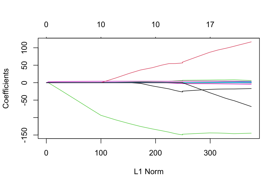
• Lasso could realize variable selection by shrinking some coefficients to exactly zero, while Ridge regression shrinks all coefficients but does not set any to zero.

R code Example of Penalized Linear Regression Models

# Install and load necessary packages
# install.packages("glmnet")
# install.packages("ISLR2")
library(glmnet)

Loading required package: Matrix

Loaded glmnet 4.1-8

library(ISLR2)

# Load the Hitters dataset
data(Hitters)

# Remove missing values
Hitters <- na.omit(Hitters)

# Define the predictor matrix and response variable
# exclude the intercept term
x <- model.matrix(Salary ~ ., Hitters)[, -1] 
y <- Hitters$Salary

# Split the data into training and test sets
set.seed(1)
train <- sample(1:nrow(x), nrow(x) / 2)
test <- (-train)
y.test <- y[test]

# Fit the Lasso model on the training data
grid <- 10^seq(10, -2, length = 100)
# LASSO-LR
lasso.mod <- glmnet(x[train, ], y[train], alpha = 1,
                    lambda = grid, family = 'gaussian')
# Plot the Lasso model to visualize coefficient paths
plot(lasso.mod)

Warning in regularize.values(x, y, ties, missing(ties), na.rm = na.rm):
collapsing to unique 'x' values

# Perform cross-validation to find the optimal lambda
set.seed(1)
cv.out <- cv.glmnet(x[train, ], y[train], alpha = 1)
plot(cv.out)

bestlam <- cv.out$lambda.min
# Make predictions on the test set using the optimal lambda
lasso.pred <- predict(lasso.mod, s = bestlam, newx = x[test, ])
test.mse <- mean((lasso.pred - y.test)^2)
print(paste("Test MSE with Lasso and optimal lambda:", test.mse))

[1] "Test MSE with Lasso and optimal lambda: 143673.618543046"

# Fit the Lasso model on the full dataset using the optimal lambda
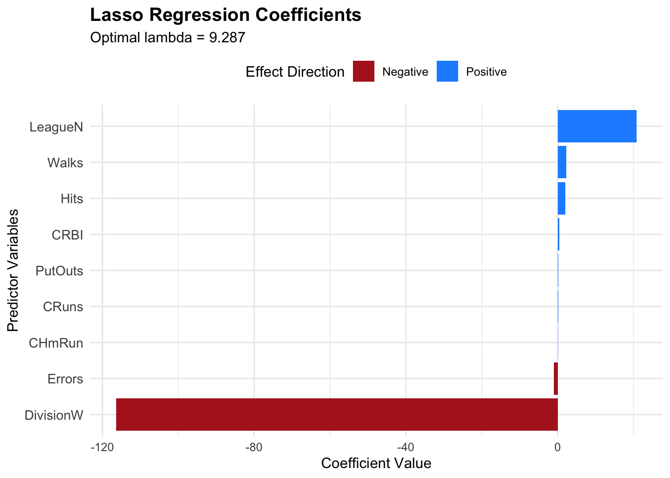
lasso.full <- glmnet(x, y, alpha = 1,lambda = bestlam)
lasso.coef <- coef(lasso.full)
print("Lasso coefficients on the full dataset:")

[1] "Lasso coefficients on the full dataset:"

print(lasso.coef)

20 x 1 sparse Matrix of class "dgCMatrix"
                       s0
(Intercept)   -3.42073206
AtBat          .         
Hits           2.02965136
HmRun          .         
Runs           .         
RBI            .         
Walks          2.24850782
Years          .         
CAtBat         .         
CHits          .         
CHmRun         0.04994886
CRuns          0.22212444
CRBI           0.40183027
CWalks         .         
LeagueN       20.83775664
DivisionW   -116.39019204
PutOuts        0.23768309
Assists        .         
Errors        -0.93567863
NewLeagueN     .         

result_matrix <- matrix(lasso.coef[lasso.coef != 0], ncol = 3, byrow = TRUE)

Warning in matrix(lasso.coef[lasso.coef != 0], ncol = 3, byrow = TRUE): data
length [10] is not a sub-multiple or multiple of the number of rows [4]

print(result_matrix)

            [,1]         [,2]      [,3]
[1,] -3.42073206    2.0296514 2.2485078
[2,]  0.04994886    0.2221244 0.4018303
[3,] 20.83775664 -116.3901920 0.2376831
[4,] -0.93567863   -3.4207321 2.0296514

# 提取非零系数（排除截距）
non_zero_coef <- lasso.coef[lasso.coef[,1] != 0, ][-1]  # 去除截距项
coef_df <- data.frame(
  Variable = names(non_zero_coef),
  Coefficient = as.numeric(non_zero_coef)
)

# 按系数绝对值排序
coef_df <- coef_df[order(abs(coef_df$Coefficient), decreasing = TRUE), ]

# 绘制条形图
library(ggplot2)

ggplot(coef_df, aes(x = reorder(Variable, Coefficient), 
                   y = Coefficient, 
                   fill = ifelse(Coefficient > 0, "Positive", "Negative"))) +
  geom_bar(stat = "identity") +
  scale_fill_manual(values = c("Positive" = "dodgerblue", "Negative" = "firebrick")) +
  labs(title = "Lasso Regression Coefficients",
       subtitle = paste("Optimal lambda =", round(bestlam, 4)),
       x = "Predictor Variables",
       y = "Coefficient Value",
       fill = "Effect Direction") +
  coord_flip() +  # 水平条形图更易阅读变量名
  theme_minimal() +
  theme(legend.position = "top",
        plot.title = element_text(face = "bold", size = 14),
        axis.text.y = element_text(size = 10))

Remark

Actually the penalized model could be applied in many regression models not only for linear regression, but also for logistic regression, Poisson regression, Cox regression, etc.

The penalized terms could be added to the loss function of these models in a similar way.

R Code of Penalized Cox Regression - Lasso using glmnet package

Want to minimize \[ -\log \left( \prod_{i:\delta_i=1} \frac{\exp\left(\sum_{j=1}^p x_{ij}\beta_j\right)}{\sum_{i':y_{i'}\geq y_i}\exp\left(\sum_{j=1}^p x_{i'j}\beta_j\right)} \right) + \lambda P(\beta), \] where \(\delta_i\) is the indicator function for censoring and \(P(\beta) = \sum_{j=1}^p \beta_j^2\) corresponds to a ridge penalty, or \(P(\beta) = \sum_{j=1}^p |\beta_j|\) corresponds to a lasso penalty.

R Code example for LASSO in Cox Regression applied on selecting important features of pesticide poisoning

Click here to see LASSO code provided by SURF2024 instructed by Dr.He

Summary

We have seen many perspectives to understand the penalized regression models, including:

• Bayes

• Lagrange multipliers

• matrix form

The greatest truths are the simplest.

Penalized regression models balance the trade-off between fitting the data well and keeping the model simple.

Everything is connected to each other. Good theory interpretes this connection interestingly.

Linear Regression: OLS and MLE

Penalized regression models: Lagrange multiplier (restriction in the geometric meaning and also algebra interpretation) and Bayesian perspective (prior: history knowledge restriction)

Background

proof of the Chebyshev’s Inequality

• Proof of the Markov’s Inequality

If \(X\) is a non-negative random variable and \(a>0\), then \[P(X\ge a) \le \frac{E(X)}{a}\] \[ E(X) = \int_{0}^{\infty} x f(x) \, dx \]

\[ E(X) = \int_{0}^{a} x f(x) \, dx + \int_{a}^{\infty} x f(x) \, dx \] \[ \int_{a}^{\infty} x f(x) \, dx \geq \int_{a}^{\infty} a f(x) \, dx = a \int_{a}^{\infty} f(x) \, dx \]

\[ E(X) \geq a \cdot P(X \geq a) \]

\[ P(X \geq a) \leq \frac{E(X)}{a} \]

• Proof of the Chebyshev’s Inequality

\[ P((X - \mu)^2 \geq k^2\sigma^2) \leq \frac{E[(X-\mu)^2]}{k^2\sigma^2}=\frac{\sigma^2}{k^2\sigma^2} = \frac{1}{k^2} \]

\[ P(|X - \mu| \geq k\sigma) \leq \frac{1}{k^2} \]

Law of Large Numbers (LLN)

• Weak Law of Large Numbers

Let \(X_1, X_2, \ldots, X_n\) be a sequence of i.i.d. random variables with finite mean \(\mu\) and finite variance \(\sigma^2\). Then for any \(\epsilon > 0\),

\[ P\left(\left|\frac{1}{n}\sum_{i=1}^{n} X_i - \mu\right| \geq \epsilon\right) \to 0 \text{ as } n \to \infty \]

• Strong Law of Large Numbers

Let \(X_1, X_2, \ldots, X_n\) be a sequence of i.i.d. random variables with finite mean \(\mu\). Then,

\[ P\left(\lim_{n \to \infty} \frac{1}{n}\sum_{i=1}^{n} X_i = \mu\right) = 1 \]

• Proof of the Weak Law of Large Numbers

By Chebyshev’s inequality, for any \(\epsilon > 0\),

\[ P\left(\left|\frac{1}{n}\sum_{i=1}^{n} X_i - \mu\right| \geq \epsilon\right) \leq \frac{\text{Var}\left(\frac{1}{n}\sum_{i=1}^{n} X_i\right)}{\epsilon^2} = \frac{\frac{1}{n^2}\cdot n\sigma^2}{\epsilon^2}=\frac{\sigma^2/n}{\epsilon^2} = \frac{\sigma^2}{n\epsilon^2} \]

As \(n \to \infty\), \(\frac{\sigma^2}{n\epsilon^2} \to 0\). Therefore, \[ P\left(\left|\frac{1}{n}\sum_{i=1}^{n} X_i - \mu\right| \geq \epsilon\right) \to 0 \text{ as } n \to \infty \]

• Proof of the Strong Law of Large Numbers (using Borel-Cantelli Lemma)

By Chebyshev’s inequality, for any \(\epsilon > 0\),

\[ P\left(\left|\frac{1}{n}\sum_{i=1}^{n} X_i - \mu\right| \geq \epsilon\right) \leq \frac{\sigma^2}{n\epsilon^2} \]

Let \(A_n = \left\{\left|\frac{1}{n}\sum_{i=1}^{n} X_i - \mu\right| \geq \epsilon\right\}\). Then,

\[ \sum_{n=1}^{\infty} P(A_n) \leq \sum_{n=1}^{\infty} \frac{\sigma^2}{n\epsilon^2} = \frac{\sigma^2}{\epsilon^2} \sum_{n=1}^{\infty} \frac{1}{n} \]

The series \(\sum_{n=1}^{\infty} \frac{1}{n}\) diverges, so we cannot directly apply the Borel-Cantelli lemma here. However, we can use a modified approach. Consider the events \(B_k = \left\{\left|\frac{1}{2^k}\sum_{i=1}^{2^k} X_i - \mu\right| \geq \epsilon\right\}\). Then,

\[ \sum_{k=1}^{\infty} P(B_k) \leq \sum_{k=1}^{\infty} \frac{\sigma^2}{2^k\epsilon^2} = \frac{\sigma^2}{\epsilon^2} \sum_{k=1}^{\infty} \frac{1}{2^k} = \frac{\sigma^2}{\epsilon^2} \]

Since \(\sum_{k=1}^{\infty} P(B_k)\) converges, by the Borel-Cantelli lemma(如果一系列独立事件的概率之和是有限的，那么这些事件无限次发生的概率为零), we have

\[ P(B_k \text{ i.o.}) = 0 \]

(i.o means infinitely often)

(p.s.: if 一系列独立事件的概率之和是无限的，并且这些事件是独立的，那么这些事件无限次发生的概率为一)

This implies that \[ P\left(\lim_{k \to \infty} \frac{1}{2^k}\sum_{i=1}^{2^k} X_i = \mu\right) = 1 \]

Now, for any \(n\), there exists a \(k\) such that \(2^k \leq n < 2^{k+1}\). We can write \[ \frac{1}{n}\sum_{i=1}^{n} X_i = \frac{1}{n}\left(\sum_{i=1}^{2^k} X_i + \sum_{i=2^k+1}^{n} X_i\right) \]

As \(k \to \infty\), the second term \(\frac{1}{n}\sum_{i=2^k+1}^{n} X_i\) becomes negligible, and we have \[ \lim_{n \to \infty} \frac{1}{n}\sum_{i=1}^{n} X_i = \mu \]

with probability 1. Therefore,

\[ P\left(\lim_{n \to \infty} \frac{1}{n}\sum_{i=1}^{n} X_i = \mu\right) = 1 \]

Central Limit Theorem (CLT)

Confidence Interval

Motivation

Statistical inference is a solution with likelihood that such solution is successful.

• Since we want the probability of the estimation and the probability of a point estimation is always 0, we need to consider the interval estimation.

• guess of \(\theta_0\) needs us to know the domain of \(\theta_0\) [L,U].

  Let the sample to be \(x_1, x_2, \ldots, x_n\) and the domain is a random interval \([L(X_1, X_2, \ldots, X_n), U(X_1, X_2, \ldots, X_n)]\) with L < U. The success is \(P(L \leq \theta_0 \leq U)=1-\alpha\).

• metaphor using the fisherman catching fish

  The fisherman wants to catch a fish with length \(\theta_0\). He uses a bamboo bucket with size [L,U] to randomly catch the fish. If the fish is in the net, then he is successful. The size of the net is random because it depends on the sample data.

  The hook is the point estimation of \(\theta_0\).

what is the good confidence interval?

Given the confidence level \(1-\alpha\), we want to find the interval [L,U] as small as possible such that \(P(L \leq \theta_0 \leq U)=1-\alpha\) to ensure the accuracy of the estimation.

Pivot—Construction of Confidence Interval

• pivot : \(T(x_1, x_2, \ldots, x_n; \theta_0) \in f(t)\). The \(\theta_0\) is apparent in the pivot

• statistics : \(T(x_1, x_2, \ldots, x_n) \in f(t; \theta_0)\). The \(\theta_0\) is hidden in the statistic so we must excavate it to get the real meaning of it.

A pivot is a function of the sample data and the parameter of interest that has a probability distribution that does not depend on the parameter. Pivots are useful for constructing confidence intervals because they allow us to make probabilistic statements about the parameter without knowing its true value.

An example using the Lagrange multiplier to minimize the size of CI given the confidence level in the senario of standard normal distribution

Getting L and U such that the confidence interval is as small as possible is a problem of minimization optimization with extra constraints.

Lagrange Multiplier Method could be used to solve the optimization problem:

Use the standard normal distribution as an example:

Want to minimize U-L subject to the constraint that \(P(L \leq \mu \leq U) = 1 - \alpha\).

\[ \phi (a,b,\lambda) = b-a + \lambda \left[ P(a \leq Z \leq b) - (1 - \alpha) \right] \]

i.e.

\[ \phi (a,b,\lambda) = b-a + \lambda (\int _{a}^{b} \frac{1}{\sqrt{2\pi}} e^{-\frac{y^2}{2}} dy - (1 - \alpha)) \]

Taking partial derivatives and setting them to zero:

\[ \frac{\partial \phi}{\partial a} = -1 + \lambda \cdot \frac{1}{\sqrt{2\pi}} e^{-\frac{a^2}{2}} = 0 \]

\[ \frac{\partial \phi}{\partial b} = 1 + \lambda \cdot \frac{1}{\sqrt{2\pi}} e^{-\frac{b^2}{2}} = 0 \]

\[ \frac{\partial \phi}{\partial \lambda} = \int _{a}^{b} \frac{1}{\sqrt{2\pi}} e^{-\frac{y^2}{2}} dy - (1 - \alpha) = 0 \]

By adding the first two equations, we get:

\[ \lambda \cdot \frac{1}{\sqrt{2\pi}} \left( e^{-\frac{a^2}{2}} - e^{-\frac{b^2}{2}} \right) = 0 \]

since \(\lambda \neq 0\), we have \(e^{-\frac{a^2}{2}} = e^{-\frac{b^2}{2}}\), which implies \(a^2 = b^2\) or \(a = -b\) (since \(a < b\)).

Therefore, for the standard normal distribution, the best confidence interval that minimizes the width \(U - L\) for a given confidence level \(1 - \alpha\) is symmetric around zero, i.e., \(L = -z_{\alpha/2}\) and \(U = z_{\alpha/2}\), where \(z_{\alpha/2}\) is the critical value from the standard normal distribution corresponding to the upper \(\alpha/2\) percentile.

Example of Confidence Interval Construction using Pivot

• Step 1: find the pivot

This should begin by standardizing.

• Step 2: find the quantiles of the pivot distribution

• Step 3: solve the inequalities to get L and U

Example 1: Confidence Interval for the exponential distribution

• step 1: find the pivot

Let \(X_1, X_2, \ldots, X_n\) be a random sample from an exponential distribution with point estimation \(\theta_0=\frac{1}{n}\sum_{i=1}^{n} X_i\). The pivot could be constructed as follows:

\[ T = \frac{1}{n}\sum_{i=1}^{n} X_i \]

method 1

Construct the pivot with the distribution of Gamma

Since \(X_i \sim \text{Exponential}(\theta_0)\), we have \[ \sum_{i=1}^{n} X_i \sim \text{Gamma}(n, \theta_0) \] Therefore, \[ \frac{\sum_{i=1}^{n} X_i}{\theta_0} \sim \text{Gamma}(n, 1) \]

method 2

By standardization, we have

\[ \frac{\frac{1}{n}\sum_{i=1}^{n} X_i-\theta_0}{ \frac{\theta_0}{\sqrt{n}}} = \frac{\sqrt{n}(\frac{1}{n}\sum_{i=1}^{n} X_i - \theta_0)}{\theta_0} \sim N(0,1) \]

Why CI is useful?

If we want to check if \(\theta_0\) is equal to a specific value \(\theta_1\), we could check if \(\theta_1\) is in the confidence interval.

(Here for the equivalence to the hypothesis testing, the null hypothesis is \(H_0: \theta_0 = \theta_1\) and the alternative hypothesis is \(H_1: \theta_0 \neq \theta_1\).)

therefore if we have constructed the \(1-\alpha\) confidence interval [L,U], then if \(\theta_1\) is not in [L,U], we say we have \(1-\alpha\) confidence to say \(\theta_0 \neq \theta_1\).

relation between CI and Hypothesis Testing

They are the same thing but they are different perspectives.

Confidence interval is a direct method to check if \(\theta_0\) is equal to a specific value \(\theta_1\). Hypothesis testing is an indirect method to check if \(\theta_0\) is equal to a specific value \(\theta_1\).

Bayesian Confidence Interval—Credible Interval

\(x_1, x_2, \ldots, x_n \sim f(x|\theta_0)\) or say \(f(x;\theta_0)\)

prior for \(\theta_0 \sim \pi(\theta)\)

\[ f(\theta|x_1,...x_n) = \frac{f(x_1,...,x_n|\theta)\pi(\theta)}{\int f(x_1,...,x_n|\theta)\pi(\theta)d\theta} \]

since they are i.i.d

\[ f(\theta|x_1,...x_n) = \frac{\prod_{i=1}^{n} f(x_i|\theta)\pi(\theta)}{\int \prod_{i=1}^{n} f(x_i|\theta)\pi(\theta)d\theta} \]

To construct the credible interval with level \(1-\alpha\), we need to find the interval [L,U] such that

\[ P(L \leq \theta_0 \leq U|x_1,...,x_n) = 1-\alpha \]

i.e.

\[ \int_{L}^{U} f(\theta|x_1,...,x_n) d\theta = 1-\alpha \]

By Lagrange Multiplier Method, we could find the best [L,U] such that U-L is as small as possible subject to the constraint.

L is the \(\alpha/2\) quantile which is the function of \(x_1,...,x_n\) and U is the \(1-\alpha/2\) quantile which is also the function of \(x_1,...,x_n\).

Bootstrap Confidence Interval

\(\theta_1, \theta_2, \ldots, \theta_B\) are the bootstrap estimates of \(\theta_0\).

\(\theta_{(1)}, \theta_{(2)}, \ldots, \theta_{(B)}\) are the order statistics of \(\theta_1, \theta_2, \ldots, \theta_B\).

therefore,

\[ (\theta_{(\alpha/2 \cdot B)}, \theta_{((1-\alpha/2) \cdot B)}) \] is the bootstrap confidence interval with level \(1-\alpha\).

Hypothesis Testing

Motivation of Hypothesis Testing

Hypothesis testing is a formal procedure for statistically evaluating whether a specific claim about a population parameter is supported by sample data.

• Proof by contradiction

The logic procedure is no direct but rater indirect, closely mirroring the proof by contradiction in mathematics.

• step 1: Assume \(A^c\) is true (null hypothesis \(H_0\) is true).

• step 2: Do a sequence of logical deductions. Once you see a clear contradiction, then you stop. (calculate the p-value)

• step 3: Conclude that \(A\) must be true (reject \(H_0\) in favor of \(H_1\)).

Then we know that hypothesis testing is the statistical version of proof by contradiction in mathematics.

However, in the mathematical proof by contradiction, the conclusion is always correct (the negation is absolutely impossible). But in hypothesis testing, there is a possibility of making errors (almost impossible \(H_0\)) since here the contradiction is just almost impossible but not absolutely impossible.

relation between CI and Hypothesis Testing (repeat here)

They are the same thing but they are different perspectives.

Confidence interval is a direct method to check if \(\theta_0\) is equal to a specific value \(\theta_1\). Hypothesis testing is an indirect method to check if \(\theta_0\) is equal to a specific value \(\theta_1\).

steps of Hypothesis Testing

How do we design a hypothesis test?

Now let us assume the population is \(N(\mu,1)\) under \(H_0\). and our goal is to prove \(\mu \neq 0\).

• Step 1: Design \(H_0\) and \(H_1\)

We always put the claim we want to prove into the alternative hypothesis \(H_1\). The opposite of the claim is put into the null hypothesis \(H_0\).

Then we do the following under the assumption that \(H_0\) is true.

Then we could design \(H_0: \mu = 0\) and \(H_1: \mu \neq 0\).

• Step 2: Design an almost impossible event C under \(H_0\).

\(X_1, X_2, \ldots, X_n\) are the random sample (i.i.d. from a common population, \(f(x;\theta)\), \(\theta \in \Theta\) parameter space).

Then the joint density of \(X_1, X_2, \ldots, X_n\) under \(H_0\) is \(f(x_1;0)f(x_2;0) \ldots f(x_n;0)\).

The chance that \(C\in R^n\) is chosen \(P((X_1, X_2, \ldots, X_n) \in C|H_0)=\int_Cf(x_1;0)f(x_2;0) \ldots f(x_n;0)dx_1dx_2 \ldots dx_n\) is very small, say less than \(\alpha\) (significance level).

Then we could design the almost impossible event C as \(|\bar{X}| > z_{\alpha/2}/\sqrt{n}\) under \(H_0\).

Do experiment and collect a data set \({x_1, x_2, \ldots, x_n}\). Do data analysis and check if \((x_1, x_2, \ldots, x_n) \in C\). If yes, then the almost impossible event happened which is a sign of contradiction, we reject \(H_0\) in favor of \(H_1\). If no, then we do not have enough evidence to reject \(H_0\).

Remark: There are many \(C\) that could be designed given \(\alpha\). Each \(C\) corresponds to a different test procedure. (So next part we will choose the best \(C\) given \(\alpha\).)

• Step 3: Conclusion

If \((x_1, x_2, \ldots, x_n) \in C\), then we reject \(H_0\) in favor of \(H_1\).

Equivalently, we accept \(H_1\) is true.

General procedure

• Step 1: Write down the statement

• Step 2: choose threshold \(\alpha\) (significance level)

• Step 3: Design an almost impossible event C under \(H_0\) such that \(P((X_1, X_2, \ldots, X_n) \in C|H_0 \text{ is true}) = \alpha\).

• Step 4: Do experiment and collect a data set \({x_1, x_2, \ldots, x_n}\).

• Step 5: check if \((x_1, x_2, \ldots, x_n) \in C\).

Do data analysis and check if \((x_1, x_2, \ldots, x_n) \in C\). If yes, then we reject \(H_0\) in favor of \(H_1\). If no, then we do not have enough evidence to reject \(H_0\) and we get no conclusion at all.

• Step 6: Conclusion

If \((x_1, x_2, \ldots, x_n) \in C\), then we reject \(H_0\) in favor of \(H_1\). Otherwise, no conclusion.

Statement

• Null hypothesis \(H_0\)

• Alternative hypothesis \(H_1\)

• Critical region C and \(\alpha\) is the size of C i.e. \(P((X_1, X_2, \ldots, X_n) \in C|H_0 \text{ is true}) = \alpha\).

Which critical region is the best?

Define the set of all critical regions with size \(\alpha\) as

\[ \mathcal{C}_{\alpha} = \{C: P((X_1, X_2, \ldots, X_n) \in C|H_0 \text{ is true}) = \alpha\} \]

First we introduce two types of mistakes in hypothesis testing:

Two types of mistakes in Hypothesis Testing

• Type I error: Rejecting \(H_0\) (because C occurs) when it is true. The probability of Type I error is \(\alpha\) i.e.\(P((X_1, X_2, \ldots, X_n) \in C|H_0 \text{ is true}) = \alpha\).

• Type II error: Not rejecting \(H_0\) (because C does not occur) when \(H_1\) is true. The probability of Type II error is \(\beta\) i.e. \(P((X_1, X_2, \ldots, X_n) \notin C|H_1 \text{ is true}) = \beta\). Here, since \(\beta\) depends on C, this gives us the creterion to choose the best C.

We say \(C_1\) is better than \(C_2\) if \(\beta(C_1) < \beta(C_2)\) given the same \(\alpha\).

\(\mathcal{C}_{\alpha}\) If \(C^*\) satisfies

\[ \beta(C^*) = \inf_{C \in \mathcal{C}_{\alpha}} \beta(C) \]

then we say \(C^*\) is the best critical region with size \(\alpha\).

Above, \(\alpha\) and \(\beta\) is complicated for medical workers to understand. So we introduce the unified function:

Unified function: Power Function

\[ K_C(\theta) = P((X_1, X_2, \ldots, X_n) \in C|\theta) \]

Here, the \(\theta\) means joint distribution of random sample \(X_1, X_2, \ldots, X_n\) which is \(f(x_1;\theta)f(x_2;\theta) \ldots f(x_n;\theta)=\int_C f(x_1;\theta)f(x_2;\theta) \ldots f(x_n;\theta)dx_1dx_2 \ldots dx_n\).

\(H_0: \theta \in \Theta_0\) and \(H_1: \theta \in \Theta_1\).

\(\Theta= \Theta_0 \cup \Theta_1\) and \(\Theta_0 \cap \Theta_1 = \emptyset\).

Then we have

\[ K_C(\theta) = \begin{cases} \alpha, & \theta \in \Theta_0 \\ 1 - \beta, & \theta \in \Theta_1 \end{cases} \]

So \(C_1\) is better than \(C_2\) if \(K_{C_1}(\theta) > K_{C_2}(\theta)\) for all \(\theta \in \Theta_1\) given the same \(\alpha\).

Example

For the above example of \(N(\mu,1)\) population, we have

\[ K_C(\mu) = P((X_1, X_2, \ldots, X_n) \in C|\mu) = \begin{cases} 0.05, & \mu = 0 \\ \int_C \prod_{i=1}^{n} \frac{1}{\sqrt{2\pi}} e^{-\frac{(x_i - \mu)^2}{2}} dx_1 dx_2 \ldots dx_n, & \mu \neq 0 \end{cases} \]

How to find the best critical region

• Simple hypothesis testing:

• Composite hypothesis testing:

Under \(H_0\) is true,

LRT

Though it might not be the most powerful test in all scenarios, the Likelihood Ratio Test (LRT) is widely used due to its general applicability and asymptotic properties.

We consider the hypotheses: \[ H_0: \theta \in \Theta_0 \quad \text{vs} \quad H_1: \theta \in \Theta_1 \] where \(\Theta_0 \cap \Theta_1 = \emptyset\) (the parameter spaces are disjoint).

Let \(X_1, \dots, X_n\) be a random sample from the distribution with PDF \(f(x; \theta)\). The likelihood function of \(\theta\) is: \[ L(\theta) = f(x_1; \theta) \cdots f(x_n; \theta) \]

The likelihood ratio \(R\) is defined as: \[ R = \frac{\sup_{\theta \in \Theta_0} L(\theta)}{\sup_{\theta \in \Theta_0 \cup \Theta_1} L(\theta)} \]

• When \(H_0\) is true, \(R \approx 1\) (since the numerator and denominator are close).

The rejection region for \(H_0\) is: \[ C = \left\{ (x_1, \dots, x_n) \in \mathbb{R}^n \mid R \leq k \right\} \] where \(k\) is a threshold determined by \(H_0\) and the significance level \(\alpha\).

Note: - \(\sup_{\theta \in \Theta_0} L(\theta) = L(\tilde{\theta})\), where \(\tilde{\theta}\) is the restricted MLE} (estimated under \(H_0\)).

• \(\sup_{\theta \in \Theta_0 \cup \Theta_1} L(\theta) = L(\hat{\theta})\), where \(\hat{\theta}\) is the full MLE} (estimated over the entire parameter space).

Thus, the likelihood ratio can also be written as: \[ R = \frac{L(\tilde{\theta})}{L(\hat{\theta})} \leq k \]

Eg. Derive the two-sample t test using the LRT

We consider two normal populations with a common unknown variance. Let the random samples be: -\(X_1, X_2, \cdots, X_n \sim N(\theta_1, \theta_3)\) -\(Y_1, Y_2, \cdots, Y_m \sim N(\theta_2, \theta_3)\)

where: -\(\theta_1, \theta_2\): Population means ((_1, _2 \() -\)_3 > 0$: Common population variance

The parameter spaces for hypotheses are:

• \[\Theta_0 = \left\{ (\theta_1, \theta_2, \theta_3) \mid \theta_1 = \theta_2, \theta_3 > 0 \right\} \quad (\text{for } H_0)\]

• \[\Theta_0 \cup \Theta_1 = \left\{ (\theta_1, \theta_2, \theta_3) \mid \theta_1, \theta_2 \in \mathbb{R}, \theta_3 > 0 \right\} \quad (\text{full parameter space})\]

We test: -\(H_0: \theta_1 = \theta_2 \quad \text{vs} \quad H_1: \theta_1 \neq \theta_2\)

step1: Likelihood & Log-Likelihood Function

The joint likelihood function of\(X_1,\cdots,X_n\) and\(Y_1,\cdots,Y_m\) is: \[ L(\theta_1, \theta_2, \theta_3) = \prod_{i=1}^n f(x_i; \theta_1, \theta_3) \prod_{j=1}^m f(y_j; \theta_2, \theta_3) \]

where the normal PDF is: \[ f(x; \mu, \sigma^2) = \frac{1}{\sqrt{2\pi \sigma^2}} \exp\left\{ -\frac{(x - \mu)^2}{2\sigma^2} \right\} \]

Substituting the normal PDF, the likelihood function becomes: \[ L(\theta_1, \theta_2, \theta_3) = \left( \frac{1}{2\pi \theta_3} \right)^{\frac{n+m}{2}} \exp\left\{ -\frac{1}{2\theta_3} \left[ \sum_{i=1}^n (x_i - \theta_1)^2 + \sum_{j=1}^m (y_j - \theta_2)^2 \right] \right\} \tag{1} \]

The corresponding log-likelihood function is: \[ \ell(\theta_1, \theta_2, \theta_3) = -\frac{n+m}{2} \log(2\pi \theta_3) - \frac{1}{2\theta_3} \left[ \sum_{i=1}^n (x_i - \theta_1)^2 + \sum_{j=1}^m (y_j - \theta_2)^2 \right] \tag{2} \]

step2: Full MLE \(\hat{\theta}\) Under \(\Theta_0 \cup \Theta_1\)

To find the full MLE\(\hat{\theta} = (\hat{\theta}_1, \hat{\theta}_2, \hat{\theta}_3)\) (no restriction\(H_0\)), solve the partial derivative system: \[ \begin{cases} \frac{\partial \ell}{\partial \theta_1} = 0 \\ \frac{\partial \ell}{\partial \theta_2} = 0 \\ \frac{\partial \ell}{\partial \theta_3} = 0 \end{cases} \]

• 2.1 Derive Full MLEs

1. Derivative w.r.t.\(\theta_1\): \[ \frac{\partial \ell}{\partial \theta_1} = \frac{1}{\theta_3} \sum_{i=1}^n (x_i - \theta_1) = 0 \implies \sum_{i=1}^n (x_i - \theta_1) = 0 \] Solving gives: \[ \hat{\theta}_1 = \frac{1}{n} \sum_{i=1}^n x_i = \bar{x} \tag{3} \]

2. Derivative w.r.t.\(\theta_2\): \[ \frac{\partial \ell}{\partial \theta_2} = \frac{1}{\theta_3} \sum_{j=1}^m (y_j - \theta_2) = 0 \implies \sum_{j=1}^m (y_j - \theta_2) = 0 \] Solving gives: \[ \hat{\theta}_2 = \frac{1}{m} \sum_{j=1}^m y_j = \bar{y} \tag{4} \]

3. Derivative w.r.t.\(\theta_3\): \[ \frac{\partial \ell}{\partial \theta_3} = -\frac{n+m}{2\theta_3} + \frac{1}{2\theta_3^2} \left[ \sum_{i=1}^n (x_i - \theta_1)^2 + \sum_{j=1}^m (y_j - \theta_2)^2 \right] = 0 \] Multiply both sides by\(2\theta_3^2\) (\(\theta_3^2 \neq 0\)): \[ -(n+m)\theta_3 + \left[ \sum_{i=1}^n (x_i - \theta_1)^2 + \sum_{j=1}^m (y_j - \theta_2)^2 \right] = 0 \] Substitute\(\hat{\theta}_1 = \bar{x}\) and\(\hat{\theta}_2 = \bar{y}\), then solve for\(\theta_3\): \[ \hat{\theta}_3 = \frac{1}{n+m} \left[ \sum_{i=1}^n (x_i - \bar{x})^2 + \sum_{j=1}^m (y_j - \bar{y})^2 \right] \tag{5} \]

• 2.2 Compute Maximized Likelihood Under Full Space ((L()$)

Substitute\(\hat{\theta}_1 = \bar{x}\),\(\hat{\theta}_2 = \bar{y}\),\(\hat{\theta}_3\) (from (3)-(5)) into the likelihood function (1): \[ L(\hat{\theta}) = \left( \frac{1}{2\pi \hat{\theta}_3} \right)^{\frac{n+m}{2}} \exp\left\{ -\frac{1}{2\hat{\theta}_3} \left[ \sum_{i=1}^n (x_i - \bar{x})^2 + \sum_{j=1}^m (y_j - \bar{y})^2 \right] \right\} \]

From equation (5), we know: \[ \sum_{i=1}^n (x_i - \bar{x})^2 + \sum_{j=1}^m (y_j - \bar{y})^2 = (n+m)\hat{\theta}_3 \]

Substitute this into the exponent term: \[ \exp\left\{ -\frac{1}{2\hat{\theta}_3} \cdot (n+m)\hat{\theta}_3 \right\} = \exp\left\{ -\frac{n+m}{2} \right\} = e^{-\frac{n+m}{2}} \]

Thus, the maximized likelihood under the full space simplifies to: \[ L(\hat{\theta}) = \left( \frac{1}{2\pi \hat{\theta}_3} \right)^{\frac{n+m}{2}} \cdot e^{-\frac{n+m}{2}} = \left( \frac{e^{-1}}{2\pi \hat{\theta}_3} \right)^{\frac{n+m}{2}} \tag{6} \]

step3: Restricted MLE (\(\tilde{\theta}\)) Under\(H_0\)

Under\(H_0: \theta_1 = \theta_2 = \theta^*\), the log-likelihood (2) simplifies to: \[ \ell(\theta^*, \theta_3) = -\frac{n+m}{2} \log(2\pi \theta_3) - \frac{1}{2\theta_3} \left[ \sum_{i=1}^n (x_i - \theta^*)^2 + \sum_{j=1}^m (y_j - \theta^*)^2 \right] \tag{7} \]

• 3.1 Derive Restricted MLEs

Solve for the restricted MLE\(\tilde{\theta} = (\tilde{\theta}^*, \tilde{\theta}_3)\):

1. Derivative w.r.t.\(\theta^*\): \[ \frac{\partial \ell}{\partial \theta^*} = \frac{1}{\theta_3} \left[ \sum_{i=1}^n (x_i - \theta^*) + \sum_{j=1}^m (y_j - \theta^*) \right] = 0 \] Since\(\theta_3 \neq 0\), the numerator must be zero: \[ \sum_{i=1}^n (x_i - \theta^*) + \sum_{j=1}^m (y_j - \theta^*) = 0 \] Expand and rearrange: \[ \sum_{i=1}^n x_i + \sum_{j=1}^m y_j - (n+m)\theta^* = 0 \] Solving gives the pooled sample mean: \[ \tilde{\theta}^* = \frac{n\bar{x} + m\bar{y}}{n+m} \tag{8} \]

2. Derivative w.r.t.\(\theta_3\): The derivative structure is the same as in Step 2.1.3. Substitute\(\theta^* = \tilde{\theta}^*\) into the derivative and set to zero: \[ \frac{\partial \ell}{\partial \theta_3} = -\frac{n+m}{2\theta_3} + \frac{1}{2\theta_3^2} \left[ \sum_{i=1}^n (x_i - \tilde{\theta}^*)^2 + \sum_{j=1}^m (y_j - \tilde{\theta}^*)^2 \right] = 0 \] Solving for\(\theta_3\) gives the restricted MLE of variance: \[ \tilde{\theta}_3 = \frac{1}{n+m} \left[ \sum_{i=1}^n (x_i - \tilde{\theta}^*)^2 + \sum_{j=1}^m (y_j - \tilde{\theta}^*)^2 \right] \tag{9} \]

• 3.2 Compute Maximized Likelihood Under\(H_0\) ((L()$)

Substitute\(\tilde{\theta}^*\) (from (8)) and\(\tilde{\theta}_3\) (from (9)) into the likelihood function (1) (under\(H_0\),\(\theta_1 = \theta_2 = \tilde{\theta}^*\)): \[ L(\tilde{\theta}) = \left( \frac{1}{2\pi \tilde{\theta}_3} \right)^{\frac{n+m}{2}} \exp\left\{ -\frac{1}{2\tilde{\theta}_3} \left[ \sum_{i=1}^n (x_i - \tilde{\theta}^*)^2 + \sum_{j=1}^m (y_j - \tilde{\theta}^*)^2 \right] \right\} \]

From equation (9), we know: \[ \sum_{i=1}^n (x_i - \tilde{\theta}^*)^2 + \sum_{j=1}^m (y_j - \tilde{\theta}^*)^2 = (n+m)\tilde{\theta}_3 \]

Substitute this into the exponent term: \[ \exp\left\{ -\frac{1}{2\tilde{\theta}_3} \cdot (n+m)\tilde{\theta}_3 \right\} = \exp\left\{ -\frac{n+m}{2} \right\} = e^{-\frac{n+m}{2}} \]

Thus, the maximized likelihood under\(H_0\) simplifies to: \[ L(\tilde{\theta}) = \left( \frac{1}{2\pi \tilde{\theta}_3} \right)^{\frac{n+m}{2}} \cdot e^{-\frac{n+m}{2}} = \left( \frac{e^{-1}}{2\pi \tilde{\theta}_3} \right)^{\frac{n+m}{2}} \tag{10} \]

step4: Likelihood Ratio Statistic

The likelihood ratio\(R\) is the ratio of the maximized likelihood under\(H_0\) to the maximized likelihood under the full space: \[ R = \frac{L(\tilde{\theta})}{L(\hat{\theta})} \]

Substitute\(L(\tilde{\theta})\) (from (10)) and\(L(\hat{\theta})\) (from (6)): \[ R = \frac{\left( \frac{e^{-1}}{2\pi \tilde{\theta}_3} \right)^{\frac{n+m}{2}}}{\left( \frac{e^{-1}}{2\pi \hat{\theta}_3} \right)^{\frac{n+m}{2}}} \]

Simplify the expression (the\(e^{-1}\) and\(2\pi\) terms cancel out): \[ R = \left( \frac{\hat{\theta}_3}{\tilde{\theta}_3} \right)^{\frac{n+m}{2}} \tag{11} \]

We reject\(H_0\) when\(R \leq k\), where\(k\) is a threshold determined by the significance level\(\alpha\) (chosen such that\(P(R \leq k \mid H_0) = \alpha\)).

step5: Transformation to Two-Sample t-Statistic

• 5.1 Define Sample Variances and Pooled Variance

First, define the unbiased sample variances for each group: \[ S_x^2 = \frac{1}{n-1}\sum_{i=1}^n (x_i - \bar{x})^2, \quad S_y^2 = \frac{1}{m-1}\sum_{j=1}^m (y_j - \bar{y})^2 \]

The pooled variance (unbiased estimate of the common population variance\(\theta_3\)) is: \[ S_p^2 = \frac{(n-1)S_x^2 + (m-1)S_y^2}{n+m-2} \tag{12} \]

• 5.2 Relate\(\hat{\theta}_3\) and\(\tilde{\theta}_3\) to Pooled Variance

From equation (5), the full MLE of variance can be rewritten using\(S_x^2\) and\(S_y^2\): \[ \hat{\theta}_3 = \frac{(n-1)S_x^2 + (m-1)S_y^2}{n+m} = \frac{(n+m-2)S_p^2}{n+m} \tag{13} \] (Substituted\(S_p^2\) from (12) into the expression.)

For the restricted MLE\(\tilde{\theta}_3\), use the identity for sum of squares: \[ \sum_{i=1}^n (x_i - \tilde{\theta}^*)^2 + \sum_{j=1}^m (y_j - \tilde{\theta}^*)^2 = \sum_{i=1}^n (x_i - \bar{x})^2 + \sum_{j=1}^m (y_j - \bar{y})^2 + \frac{nm}{n+m}(\bar{x} - \bar{y})^2 \] This is the “sum of squares decomposition” (total SS = within-group SS + between-group SS). Substitute into equation (9): \[ \tilde{\theta}_3 = \frac{(n-1)S_x^2 + (m-1)S_y^2 + \frac{nm}{n+m}(\bar{x} - \bar{y})^2}{n+m} \] Using (13), substitute\((n-1)S_x^2 + (m-1)S_y^2 = (n+m)\hat{\theta}_3\): \[ \tilde{\theta}_3 = \frac{(n+m)\hat{\theta}_3 + \frac{nm}{n+m}(\bar{x} - \bar{y})^2}{n+m} = \hat{\theta}_3 + \frac{nm}{(n+m)^2}(\bar{x} - \bar{y})^2 \tag{14} \]

• 5.3 Derive the t-Statistic Relationship

Substitute (13) and (14) into the likelihood ratio (11): \[ R = \left( \frac{\hat{\theta}_3}{\hat{\theta}_3 + \frac{nm}{(n+m)^2}(\bar{x} - \bar{y})^2} \right)^{\frac{n+m}{2}} \]

Divide numerator and denominator inside the parentheses by\(\hat{\theta}_3\): \[ R = \left( \frac{1}{1 + \frac{nm}{(n+m)^2 \hat{\theta}_3}(\bar{x} - \bar{y})^2} \right)^{\frac{n+m}{2}} \]

From (13),\(\hat{\theta}_3 = \frac{(n+m-2)S_p^2}{n+m}\). Substitute this into the expression: \[ \frac{nm}{(n+m)^2 \hat{\theta}_3} = \frac{nm}{(n+m)^2 \cdot \frac{(n+m-2)S_p^2}{n+m}} = \frac{nm}{(n+m)(n+m-2)S_p^2} \]

Thus: \[ R = \left( \frac{1}{1 + \frac{nm(\bar{x} - \bar{y})^2}{(n+m)(n+m-2)S_p^2}} \right)^{\frac{n+m}{2}} \]

Notice that the term inside the parentheses can be rewritten using the two-sample t-statistic. The t-statistic is defined as: \[ T = \frac{\bar{x} - \bar{y}}{S_p \sqrt{\frac{1}{n} + \frac{1}{m}}} = \frac{\bar{x} - \bar{y}}{S_p \sqrt{\frac{n+m}{nm}}} \]

Square both sides to get\(T^2\): \[ T^2 = \frac{nm(\bar{x} - \bar{y})^2}{(n+m)S_p^2} \]

Substitute\(T^2\) into the expression for\(R\): \[ R = \left( \frac{1}{1 + \frac{T^2}{n+m-2}} \right)^{\frac{n+m}{2}} = \left( 1 + \frac{T^2}{n+m-2} \right)^{-\frac{n+m}{2}} \tag{15} \]

• 5.4 Rejection Region in Terms of t-Statistic

We reject\(H_0\) when\(R \leq k\). From (15), this is equivalent to: \[ \left( 1 + \frac{T^2}{n+m-2} \right)^{-\frac{n+m}{2}} \leq k \]

Take the reciprocal of both sides (reversing the inequality): \[ \left( 1 + \frac{T^2}{n+m-2} \right)^{\frac{n+m}{2}} \geq \frac{1}{k} \]

Raise both sides to the power of\(\frac{2}{n+m}\): \[ 1 + \frac{T^2}{n+m-2} \geq \left( \frac{1}{k} \right)^{\frac{2}{n+m}} \]

Let\(C = \left( \frac{1}{k} \right)^{\frac{2}{n+m}} - 1\) (a positive constant), then: \[ \frac{T^2}{n+m-2} \geq C \implies T^2 \geq C(n+m-2) \]

Let\(C' = \sqrt{C(n+m-2)}\), the rejection region becomes: \[ |T| \geq C' \]

Under\(H_0\), the t-statistic\(T \sim t(n+m-2)\) (t-distribution with\(n+m-2\) degrees of freedom). Thus,\(C'\) is the critical value from the t-distribution such that\(P(|T| \geq C' \mid H_0) = \alpha\).

bias- variance trade-off

\[ MSE=Var+Bias^2 \]