Chi-square
Chi-square is a
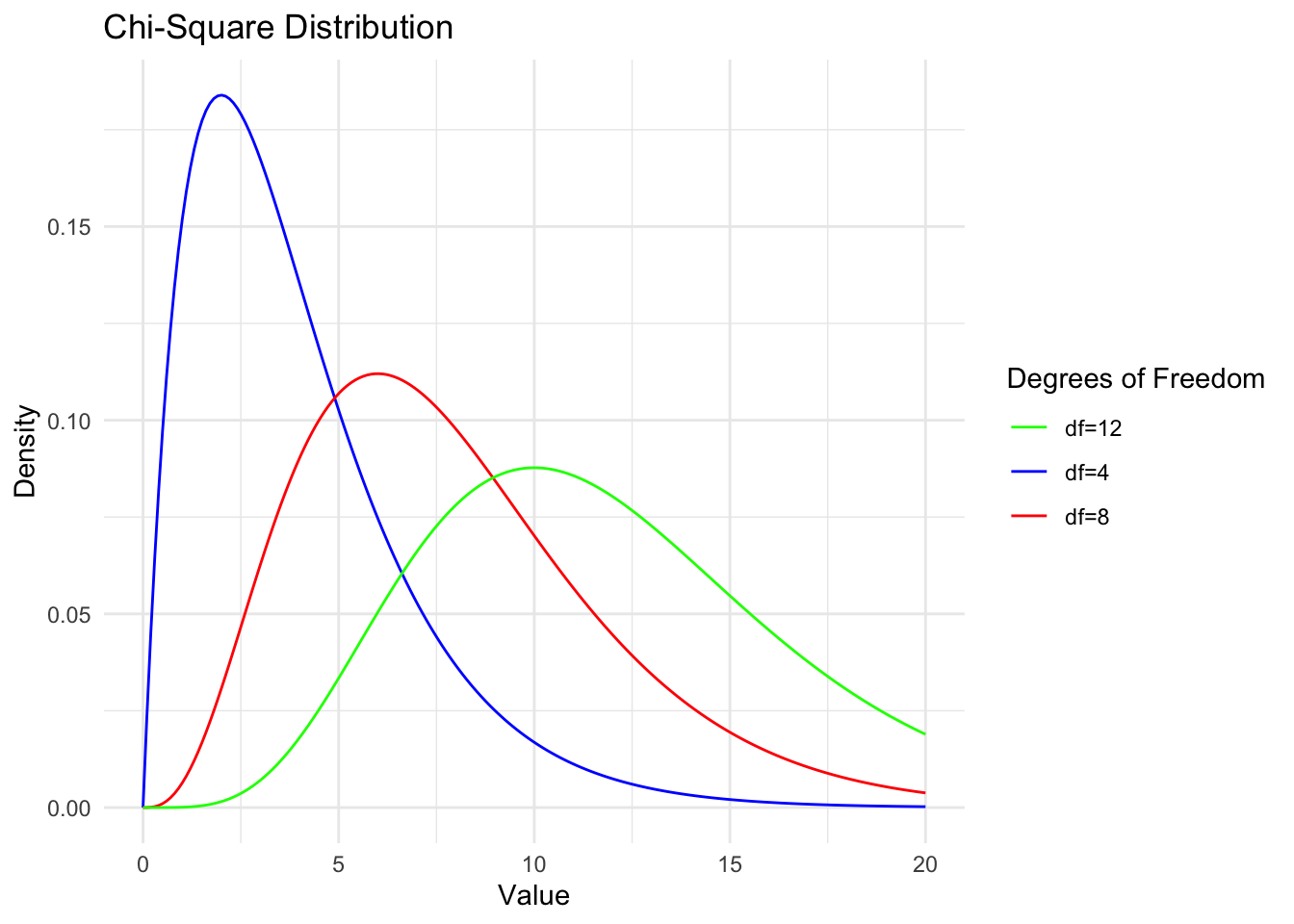
1.Let ( \(Z_1\), \(Z_2\), , \(Z_i\) ) are independent standard normal random variables(i.e. Z~N(0,1)), then the random variable ( X ) defined by
\[
X = Z_1^2 + Z_2^2 + \cdots + Z_i^2
\] (\(Z_j\)~iid.N(0,1))
follows a chi-square distribution with ( i ) degrees of freedom. So chi-square of 1 is the same thing as Gamma of (1/2,1/2) so chi-square of n is Gamma(n/2,1/2)
2.If \[
Z_i = \frac{x_i - \mu}{\sigma}
\] The sum of squared standardized deviations is:
\[
\sum_{i=1}^n Z_i^2 = \sum_{i=1}^n \left( \frac{x_i - \mu}{\sigma} \right)^2 = \frac{1}{\sigma^2} \sum_{i=1}^n (x_i - \mu)^2
\]
Let \(x_1, x_2, \cdots, x_n\) be samples of \(N\left(\mu, \sigma^2\right)\) , \(\mu\) is a known constant, find the distribution of statistics: \[
T=\sum_{i=1}^n\left(x_i-\mu\right)^2
\]
sol: \(y_i=\left(x_i-\mu\right) / \sigma, i=1,2, \cdots, n\), 则 \(y_1, y_2, \cdots, y_n\) are iid r.v. of \(N(0,1)\),so\[
\frac{T}{\sigma^2}=\sum_{i=1}^n\left(\frac{x_i-\mu}{\sigma}\right)^2=\sum_{i=1}^n y_i^2 \sim \chi^2(n),
\] (i.e.\[
\sum_{i=1}^n Z_i^2 {\sigma^2}\sim \chi^2(n)\])
Besides, \(T\)’s PDF is \[
p(t)=\frac{1}{\left(2 \sigma^2\right)^{n / 2} \Gamma(n / 2)} \mathrm{e}^{-\frac{1}{2 \sigma^2} t^{\frac{n}{2}}-1}, \quad t>0,
\]
which is Gamma distribution \(G a\left(\frac{n}{2}, \frac{1}{2 \sigma^2}\right) \cdot\)
3.chi-square is uesful because of theorems below:let \(x_1, x_2, \cdots, x_n\) are samples from \(N\left(\mu, \sigma^2\right)\) , whose sample mean and sample variance are\[
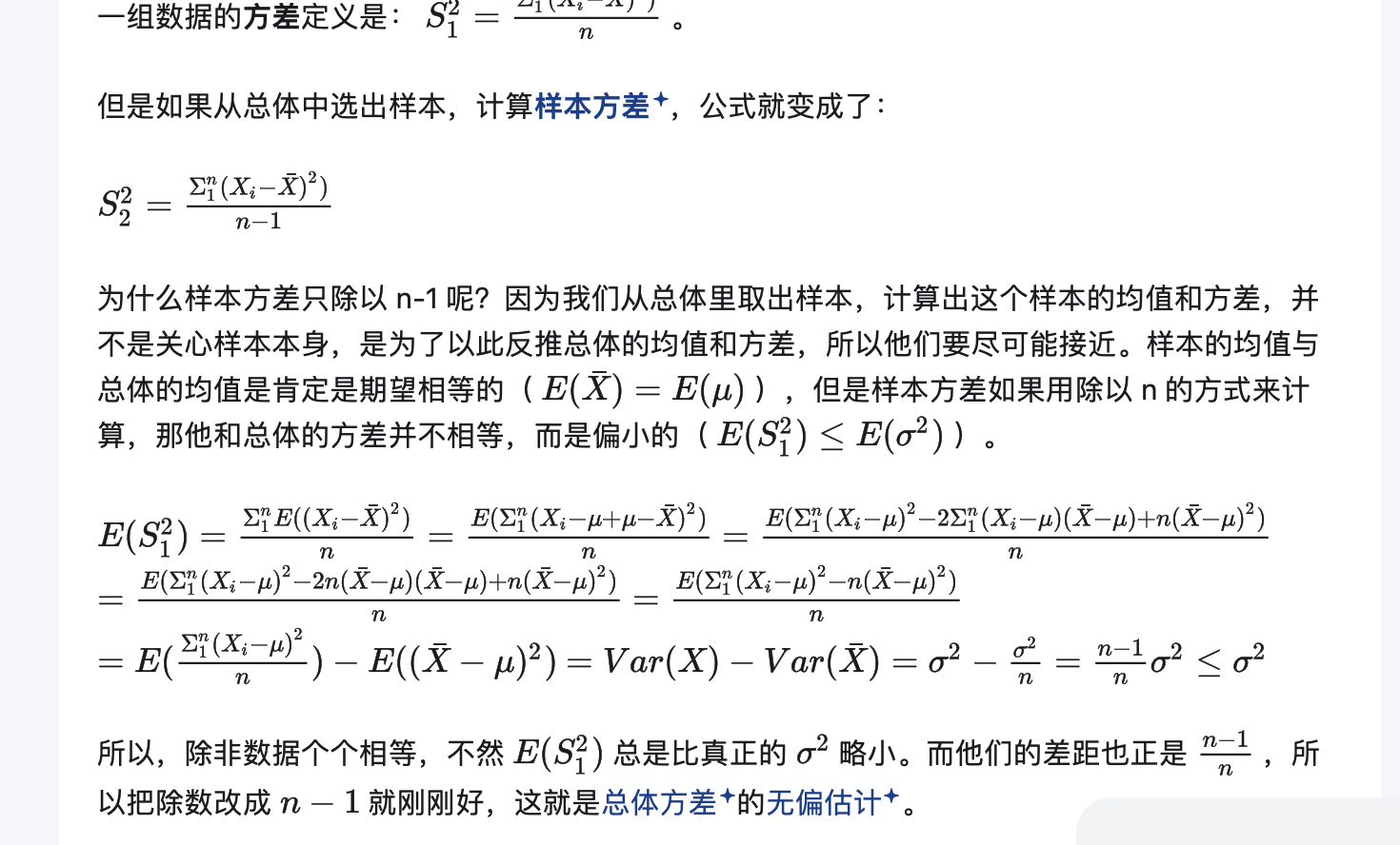
\bar{x}=\frac{1}{n} \sum_{i=1}^n x_i \text { and } s^2=\frac{1}{n-1} \sum_{i=1}^n\left(x_i-\bar{x}\right)^2,
\]
then we can get: (1) \(\bar{x}\) and \(s^2\) are independent; (2) \(\bar{x} \sim N\left(\mu, \sigma^2 / n\right)\); (3) \(\frac{(n-1) s^2}{\sigma^2} \sim \chi^2(n-1)\).
Proof: \[
p\left(x_1, x_2, \cdots, x_n\right)=\left(2 \pi \sigma^2\right)^{-n / 2} \mathrm{e}^{-\sum_{i=1}^n \frac{\left(x_i-\mu\right)^2}{2 \sigma^2}}=\left(2 \pi \sigma^2\right)^{-n / 2} \exp \left\{-\frac{\sum_{i=1}^n x_i^2-2 n \bar{x} \mu+n \mu^2}{2 \sigma^2}\right\}
\]
denote\(\boldsymbol{X}=\left(x_1, x_2, \cdots, x_n\right)^{\mathrm{T}}\), then we create an \(n\)-dimension orthogonal \(\boldsymbol{A}\) and every element in the first row is \(1 / \sqrt{n}\), such as \[
A=\left(\begin{array}{ccccc}
\frac{1}{\sqrt{n}} & \frac{1}{\sqrt{n}} & \frac{1}{\sqrt{n}} & \cdots & \frac{1}{\sqrt{n}} \\
\frac{1}{\sqrt{2 \cdot 1}} & -\frac{1}{\sqrt{2 \cdot 1}} & 0 & \cdots & 0 \\
\frac{1}{\sqrt{3 \cdot 2}} & \frac{1}{\sqrt{3 \cdot 2}} & -\frac{2}{\sqrt{3 \cdot 2}} & \cdots & 0 \\
\vdots & \vdots & \vdots & & \vdots \\
\frac{1}{\sqrt{n(n-1)}} & \frac{1}{\sqrt{n(n-1)}} & \frac{1}{\sqrt{n(n-1)}} & \cdots & -\frac{n-1}{\sqrt{n(n-1)}}
\end{array}\right),
\] 令 \(\boldsymbol{Y}=\left(y_1, y_2, \cdots, y_n\right)^{\mathrm{T}}=\boldsymbol{A} \boldsymbol{X}\), \(|Jacobi|=1\), and we can find thatt\[
\begin{gathered}
\bar{x}=\frac{1}{\sqrt{n}} y_1, \\
\sum_{i=1}^n y_i^2=\boldsymbol{Y}^{\mathrm{T}} \boldsymbol{Y}=\boldsymbol{X}^{\mathrm{T}} \boldsymbol{A}^{\mathrm{T}} \boldsymbol{A} \boldsymbol{X}=\sum_{i=1}^n x_i^2,
\end{gathered}
\]
so\(y_1, y_2, \cdots, y_n\) ’s joint density function is \[
\begin{aligned}
p\left(y_1, y_2, \cdots, y_n\right) & =\left(2 \pi \sigma^2\right)^{-n / 2} \exp \left\{-\frac{\sum_{i=1}^n y_i^2-2 \sqrt{n} y_1 \mu+n \mu^2}{2 \sigma^2}\right\} \\
& =\left(2 \pi \sigma^2\right)^{-n / 2} \exp \left\{-\frac{\sum_{i=2}^n y_i^2+\left(y_1-\sqrt{n} \mu\right)^2}{2 \sigma^2}\right\}
\end{aligned}
\]
So, \(\boldsymbol{Y}=\left(y_1, y_2, \cdots, y_n\right)^{\mathrm{T}}\) independently distributed as normal distribution and their variances are all equal to\(\sigma^2\), but their means are not all the same because \(y_2, \cdots, y_n\) ’s means are \(0, y_1\)’s is \(\sqrt{n} \mu\), which ends our proof of (2). \[
(n-1) s^2=\sum_{i=1}^n\left(x_i-\bar{x}\right)^2=\sum_{i=1}^n x_i^2-(\sqrt{n} \bar{x})^2=\sum_{i=1}^n y_i^2-y_1^2=\sum_{i=2}^n y_i^2,
\]
This proves conclusion (1). Since \(y_2, \cdots, y_n\) are independently and identically distributed as \(N\left(0, \sigma^2\right)\), we have: \[
\frac{(n-1) s^2}{\sigma^2}=\sum_{i=2}^n\left(\frac{y_i}{\sigma}\right)^2 \sim \chi^2(n-1) .
\]
Theorem is proved. (similar to the proof above this maybe easier to understand:\(\begin{aligned} & i z\left(Y_1, Y_2, \cdots, Y_2\right)^{\top}=A\left(X_1, \cdots, x_n\right)^{\top} \\ & \text { then } \sum_{i=1}^n Y_i^2=\left(Y_1, \cdots, Y_n\right)\left(Y_1, \cdots, Y_n\right)^{\top} \\ & =\left[A\left(x_1, \cdots, x_n\right)^{\top}\right]^{\top}\left[A\left(x_1, \cdots, X_n\right)^{\top}\right] \\ & =\left(x_1, \cdots, x_n\right) A^{\top} A\left(x_1, \cdots, x_n\right)^{\top} \\ & =\left(x_1, \cdots, x_n\right) E\left(x_1, \cdots, x_n\right)^{\top}=\sum_{i=1}^n x_i^2 \\ & \end{aligned}\)) \(\begin{aligned} & \text { besides } Y_1=\frac{1}{\sqrt{n}} x_1+\cdots+\frac{1}{\sqrt{n}} x_n=\frac{1}{\sqrt{n}} \sum_{i=1}^n X_i \\ & \text { and } Y_1=\sqrt{n} \cdot \frac{1}{n} \sum_{i=1}^n X_i=\sqrt{n} \bar{X}, \text { then } \bar{x}=\frac{1}{\sqrt{n}} y_i \\ & B S^2=\frac{1}{n-1} \sum_{i=1}^n\left(x_i-\bar{x}\right)^2=\frac{1}{n-1}\left[\sum_{i=1}^n x_i^2-n \bar{x}^2\right] \\ & =\frac{1}{n-1}\left[\sum_{i=1}^n Y_i^2-Y_1^2\right]=\frac{1}{n-1} \sum_{i=2}^n Y_i^2 \\ & 2 \oplus L=(\sqrt{2 \pi} \sigma)^{-n} \exp \left[-\frac{1}{2 \sigma^2} \sum_{i=1}^n\left(x_i-\mu\right)^2\right] \text {. } \\ & =(\sqrt{2 \pi} \sigma)^{-n} \exp \left[-\frac{1}{2 \sigma^2}\left(\sum_{i=1}^n x_i^2-2 \mu n \bar{x}+\mu^2 n\right]\right. \\ & =(\sqrt{2 \pi} \sigma)^{-n} \exp \left[-\frac{1}{2 \sigma^2}\left(\sum_{1=1}^n y_i{ }^2-2 \mu n \frac{1}{\sqrt{n}} Y_1+n \mu^2\right]\right. \\ & \end{aligned}\) \[=(\sqrt2\pi\sigma)^{-1}exp[-1/2\sigma^2(Y_1-\sqrt nu)^2]×(\sqrt2\pi\sigma)^{-1}exp[-1/2\sigma^2{Y_2}^2]*...*(\sqrt2\pi\sigma)^{-1}exp[-1/2\sigma^2{Y_n}^2]
\]
So L is \(Y_1\)…\(Y_n\)’s joint density function and so they are independent. Besides, we have proved that its mean is \(1/\sqrt n\)\(Y_1\) and \(S^2\)=\(1/n-1 \Sigma{i=2}Y_i^2\), so the normal distribution’s mean and variance are independent.
When the random variable \(\chi^2 \sim \chi^2(n)\), for a given \(\alpha\) (where \(0<\) \(\alpha<1\) ), the value \(\chi_{1-\alpha}^2(n)\) satisfying the probability equation \(P\left(\chi^2 \leqslant \chi_{1-\alpha}^2(n)\right)=1-\) \(\alpha\) is called the \(1-\alpha\) quantile of the \(\chi^2\) distribution with \(n\) degrees of freedom.
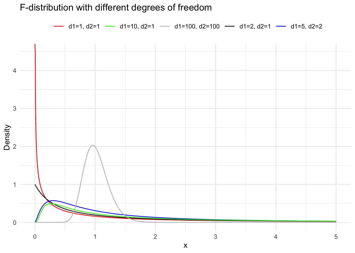
Suppose the random variables \(X_1 \sim \chi^2(m)\) and \(X_2 \sim \chi^2(n)\), and \(X_1\) and \(X_2\) are independent. Then the distribution of \(F=\frac{X_1 / m}{X_2 / n}\) is called the \(\mathrm{F}\) distribution with \(m\) and \(n\) degrees of freedom, denoted as \(F \sim F(m, n)\). Here, \(m\) is called the numerator degrees of freedom and \(n\) the denominator degrees of freedom. We derive the density function of the \(\mathrm{F}\) distribution in two steps. First, we derive the density function of \(Z=\frac{X_1}{X_2}\). Let \(p_1(x)\) and \(p_2(x)\) be the density functions of \(\chi^2(m)\) and \(\chi^2(n)\) respectively. According to the formula for the distribution of the quotient of independent random variables, the density function of \(Z\) is: \[
\begin{gathered}
p_Z(z)=\int_0^{\infty} x_2 p_1\left(z x_2\right) p_2\left(x_2\right) \mathrm{d} x_2 \\
=\frac{z^{\frac{m}{2}-1}}{\Gamma\left(\frac{m}{2}\right) \Gamma\left(\frac{n}{2}\right) 2^{\frac{m+n}{2}}} \int_0^{\infty} x_2^{\frac{n}{2}-1} e^{-\frac{x_2}{2}(1+z)} \mathrm{d} x_2 .
\end{gathered}
\]
Using the transformation \(u=\frac{x_2}{2}(1+z)\), we get: \[
p_Z(z)=\frac{z^{\frac{m}{2}-1}(1+z)^{-\frac{m+n}{2}}}{\Gamma\left(\frac{m}{2}\right) \Gamma\left(\frac{n}{2}\right)} \int_0^{\infty} u^{\frac{n}{2}-1} e^{-u} \mathrm{~d} u
\]
The final integral is the gamma function \(\Gamma\left(\frac{n}{2}\right)\), so: \[
p_Z(z)=\frac{\Gamma\left(\frac{m+n}{2}\right)}{\Gamma\left(\frac{m}{2}\right) \Gamma\left(\frac{n}{2}\right)} z^{\frac{m}{2}-1}(1+z)^{-\frac{m+n}{2}}, \quad z \geq 0 .
\]
Second, we derive the density function of \(F=\frac{n}{m} Z\). Let the value of \(F\) be \(y\). For \(y \geq 0\), we have: \[
\begin{aligned}
p_F(y) & =p_Z\left(\frac{m}{n} y\right) \cdot \frac{m}{n}=\frac{\Gamma\left(\frac{m+n}{2}\right)}{\Gamma\left(\frac{m}{2}\right) \Gamma\left(\frac{n}{2}\right)}\left(\frac{m}{n} y\right)^{\frac{m}{2}-1}\left(1+\frac{m}{n} y\right)^{-\frac{m+n}{2}} \cdot \frac{m}{n} \\
& =\frac{\Gamma\left(\frac{m+n}{2}\right)}{\Gamma\left(\frac{m}{2}\right) \Gamma\left(\frac{n}{2}\right)}\left(\frac{m}{n}\right)\left(\frac{m}{n} y\right)^{\downarrow \frac{2}{2}-1}\left(1+\frac{m}{n} y\right)^{-\frac{m+n}{2}}
\end{aligned}
\]
When the random variable \(F \sim F(m, n)\), for a given \(\alpha\) (where \(0<\alpha<1\) ), the value \(F_{1-\alpha}(m, n)\) satisfying the probability equation \(P\left(F \leqslant F_{1-\alpha}(m, n)\right)=1-\alpha\) is called the \(1-\alpha\) quantile of the \(\mathrm{F}\) distribution with \(m\) and \(n\) degrees of freedom. By the construction of the \(\mathrm{F}\) distribution, if \(F \sim F(m, n)\), then \(1 / F \sim F(n, m)\). Therefore, for a given \(\alpha\) (where \(0<\alpha<1\) ), \[
\alpha=P\left(\frac{1}{F} \leqslant F_\alpha(n, m)\right)=P\left(F \geqslant \frac{1}{F_\alpha(n, m)}\right) .
\]
Thus, \[
P\left(F \leqslant \frac{1}{F_\alpha(n, m)}\right)=1-\alpha
\]
This implies \[
F_\alpha(n, m)=\frac{1}{F_{1-\alpha}(m, n)} .
\]
Corollary Suppose \(x_1, x_2, \cdots, x_m\) is a sample from \(N\left(\mu_1, \sigma_1^2\right)\) and \(y_1, y_2, \cdots, y_n\) is a sample from \(N\left(\mu_2, \sigma_2^2\right)\), and these two samples are independent. Let: \[
s_x^2=\frac{1}{m-1} \sum_{i=1}^m\left(x_i-\bar{x}\right)^2, \quad s_y^2=\frac{1}{n-1} \sum_{i=1}^n\left(y_i-\bar{y}\right)^2,
\] where \[
\bar{x}=\frac{1}{m} \sum_{i=1}^m x_i, \quad \bar{y}=\frac{1}{n} \sum_{i=1}^n y_i
\] then \[
F=\frac{s_x^2 / \sigma_1^2}{s_y^2 / \sigma_2^2} \sim F(m-1, n-1) .
\]
In particular, if \(\sigma_1^2=\sigma_2^2\), then \(F=\frac{s_x}{s_y^2} \sim F(m-1, n-1)\). Proof: Since the two samples are independent, \(s_x^2\) and \(s_y^2\) are independent. According to a Theorem , we have \[
\frac{(m-1) s_x^2}{\sigma_1^2} \sim \chi^2(m-1), \quad \frac{(n-1) s_y^2}{\sigma_2^2} \sim \chi^2(n-1) .
\]
By the definition of the \(\mathrm{F}\) distribution, \(F \sim F(m-1, n-1)\). Corollary: Suppose \(x_1, x_2, \cdots, x_n\) is a sample from a normal distribution \(N\left(\mu, \sigma^2\right)\), and let \(\bar{x}\) and \(s^2\) denote the sample mean and sample variance of the sample, respectively. Then \[
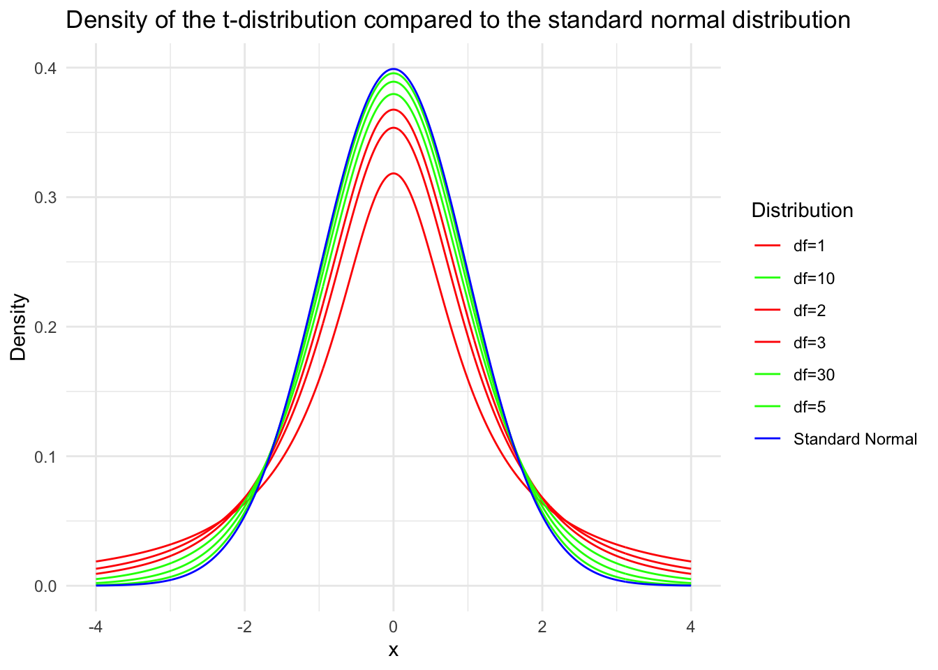
t=\frac{\sqrt{n}(\bar{x}-\mu)}{s} \sim t(n-1) .
\]
Proof: From a Theorem we obtain \[
\frac{\bar{x}-\mu}{\sigma / \sqrt{n}} \sim N(0,1)
\]
Then, \[
\frac{\sqrt{n}(\bar{x}-\mu)}{s}=\frac{\frac{\bar{x}-\mu}{\sigma / \sqrt{n}}}{\sqrt{\frac{(n-1) s^2 / \sigma^2}{n-1}}}
\]
Since the numerator is a standard normal variable and the denominator’s square root contains a \(\chi^2\) variable with \(n-1\) degrees of freedom divided by its degrees of freedom, and they are independent, by the definition of the \(t\) distribution, \(t \sim t(n-1)\). The proof is complete.
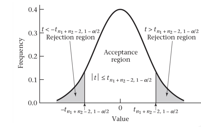
Corollary: In the notation of Corollary , assume \(\sigma_1^2=\sigma_2^2=\sigma^2\), and let \[
s_w^2=\frac{(m-1) s_x^2+(n-1) s_y^2}{m+n-2}=\frac{\sum_{i=1}^m\left(x_i-\bar{x}\right)^2+\sum_{i=1}^n\left(y_i-\bar{y}\right)^2}{m+n-2}
\]
Then \[
\frac{(\bar{x}-\bar{y})-\left(\mu_1-\mu_2\right)}{s_w \sqrt{\frac{1}{m}+\frac{1}{n}}} \sim t(m+n-2)
\]
Proof: Since \(\bar{x} \sim N\left(\mu_1, \frac{\sigma^2}{m}\right), \bar{y} \sim N\left(\mu_2, \frac{\sigma^2}{n}\right)\), and \(\bar{x}\) and \(\bar{y}\) are independent, we have
\[
\bar{x}-\bar{y} \sim N\left(\mu_1-\mu_2,\left(\frac{1}{m}+\frac{1}{n}\right) \sigma^2\right) .
\]
Thus, \[
\frac{(\bar{x}-\bar{y})-\left(\mu_1-\mu_2\right)}{\sigma \sqrt{\frac{1}{m}+\frac{1}{n}}} \sim N(0,1) .
\]
By a Theorem , we know that \(\frac{(m-1) s_x^2}{\sigma^2} \sim \chi^2(m-1)\) and \(\frac{(n-1) s_y^2}{\sigma^2} \sim \chi^2(n-1)\), and they are independent. By additivity, we have \[
\frac{(m+n-2) s_w^2}{\sigma^2}=\frac{(m-1) s_x^2+(n-1) s_y^2}{\sigma^2} \sim \chi^2(m+n-2) .
\]
Since \(\bar{x}-\bar{y}\) and \(s_w^2\) are independent, by the definition of the \(\mathrm{t}\) distribution, we get the desired result. \(\square\)
One interesting example shows the relationship of above distributions used charismatically to solve problems: r.v.: \(X_1 , X_2 , X_3 , X_4\) indpendently identically distribute(iid) as \(N\left(0 . \sigma^2\right)\). \(Z=\left(x_1^2+x_2^2\right) /\left(x_1^2+x_2^2+x_3^2+x_4^2\right)\) prove: \(Z \sim U(0.1)\). \[
\begin{aligned}
& \text { Solution: } Let Y=\frac{X_3^2+X_4^2}{X_1^2+X_2^2}=\frac{\left[\left(\frac{X_3}{\sigma}\right)^2+\left(\frac{X_4}{\sigma}\right)^2\right] / 2}{\left[\left(\frac{X_1}{\sigma}\right)^2+\left(\frac{X_2}{\sigma}\right)^2\right] / 2} \sim F(2,2) . \\
& \text { i.e. } f_Y(y)=\frac{1}{(1+y)^2}, y>0 \\
& \text { then } P(Z \leq z)=P\left(\frac{1}{1+Y} \leq z\right)=P\left(Y \geqslant \frac{1}{z}-1\right) \\
& =\int_{\frac{1}{z}-1}^{+\infty} \frac{1}{(1+y)^2} d y=z \quad \text { H } 0<z<1 . \\
& \therefore Z \sim U(0.1)
\end{aligned}
\] (ps:$
\[\begin{aligned} & f(x)=\frac{\Gamma\left(\frac{n_1+n_2}{2}\right)}{\Gamma\left(\frac{n_2}{2}\right) \Gamma\left(\frac{n_1}{2}\right)}\left(\frac{n_1}{n_2}\right)\left(\frac{n_1}{n_2} x\right)^{\frac{n_1}{2}-1}\left(1+\frac{n_1}{n_2} x\right)^{\frac{-1}{2}\left(n_1+n_2\right)} . \\ & \text { of these } x>0 \text {. and } E(x)=\frac{n_2}{n_2-2} \text {, when } n_2>2 \text {. } \\ & \operatorname{Var}(X)=\frac{2 n_2^2\left(n_1+n_2-2\right)}{n_1\left(n_2-2\right)^2\left(n_2-4\right)} \text {when $n_2>4$. } \\ & \end{aligned}\]


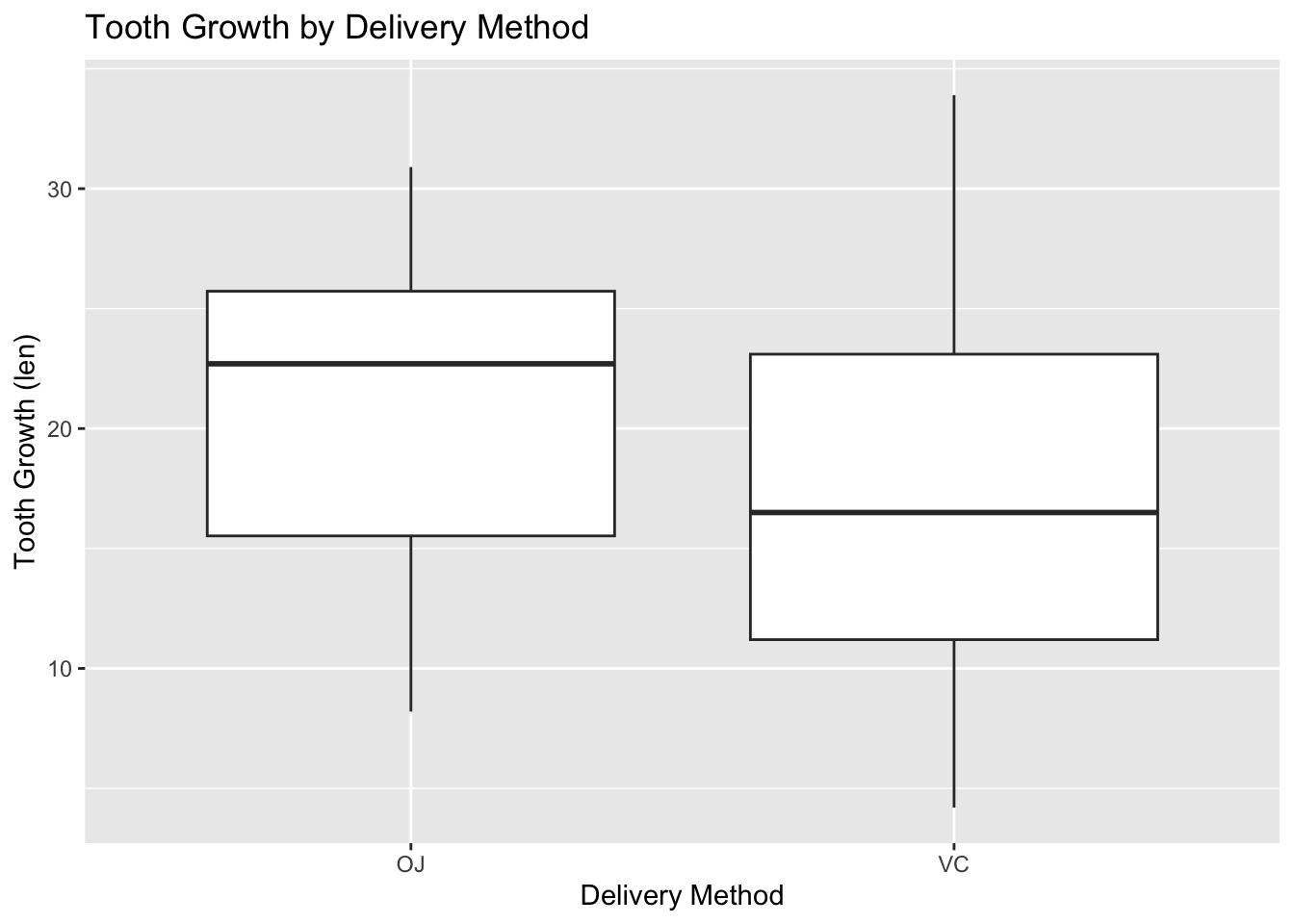
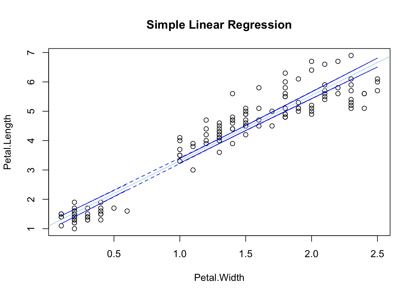
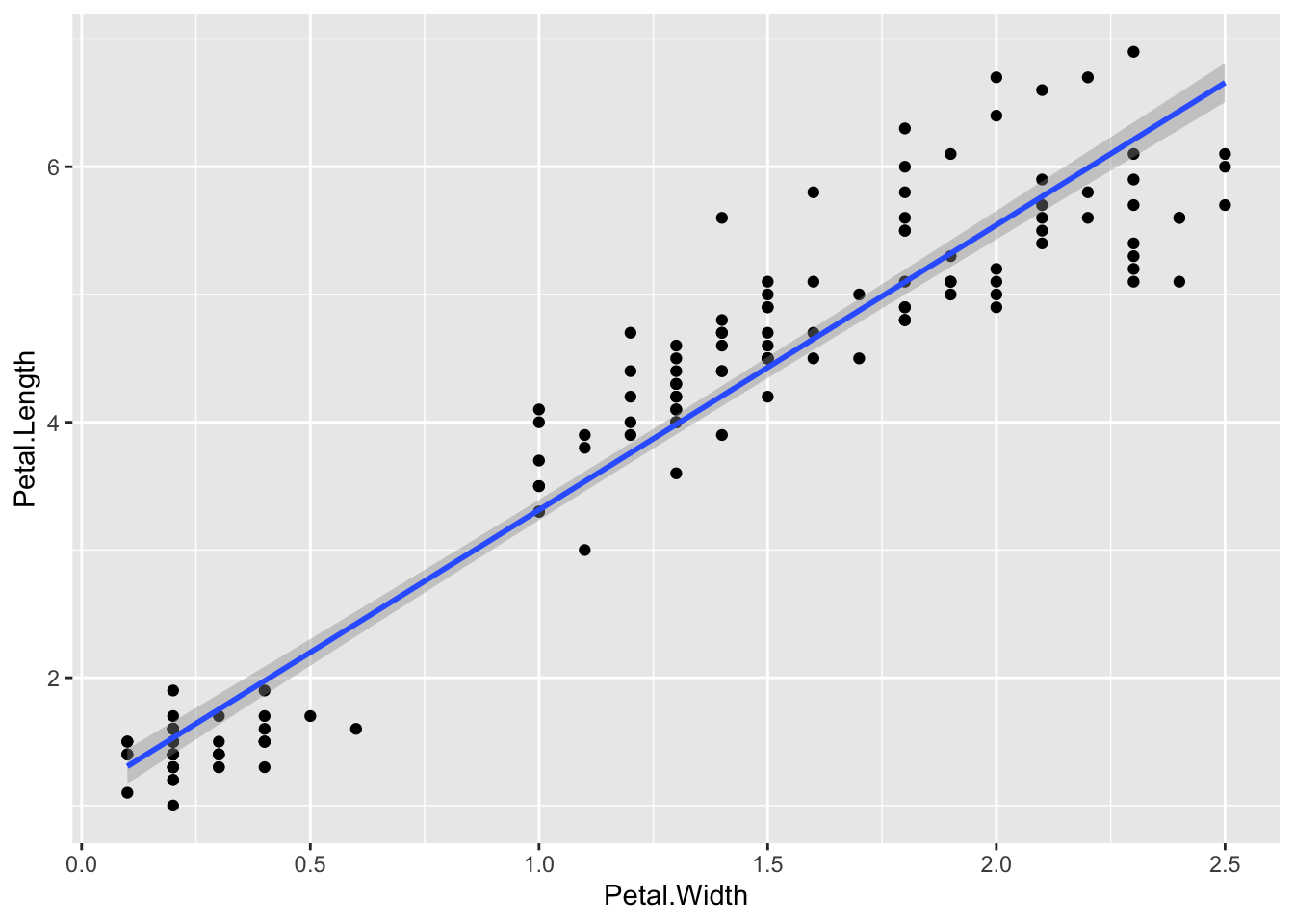


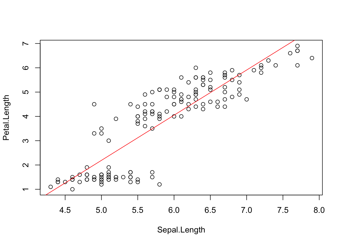


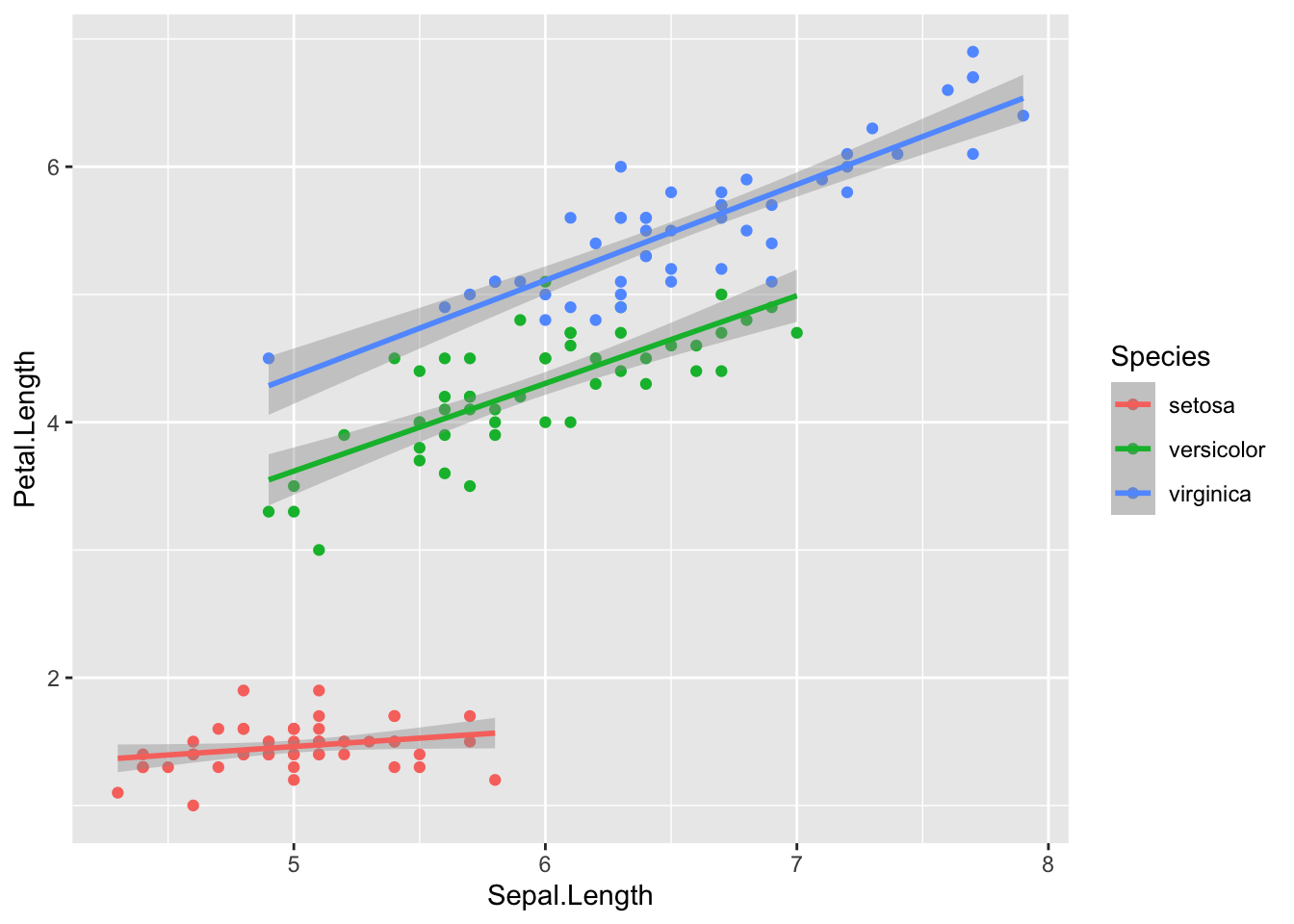


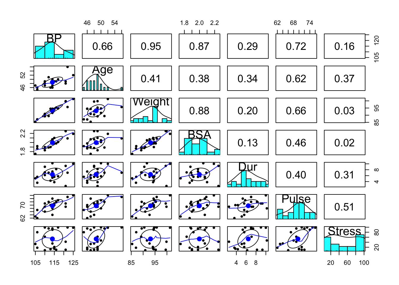


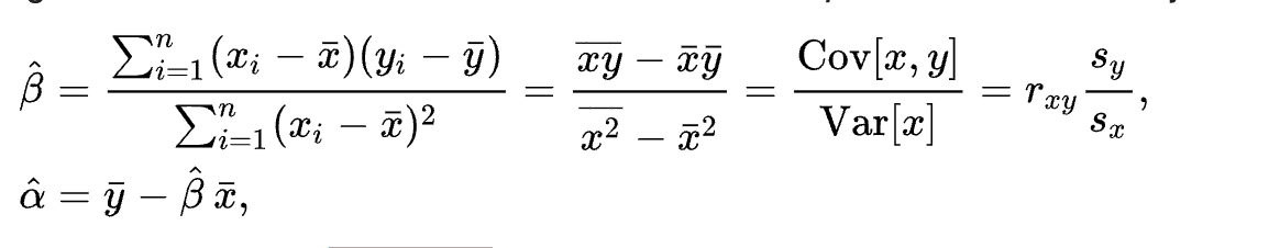
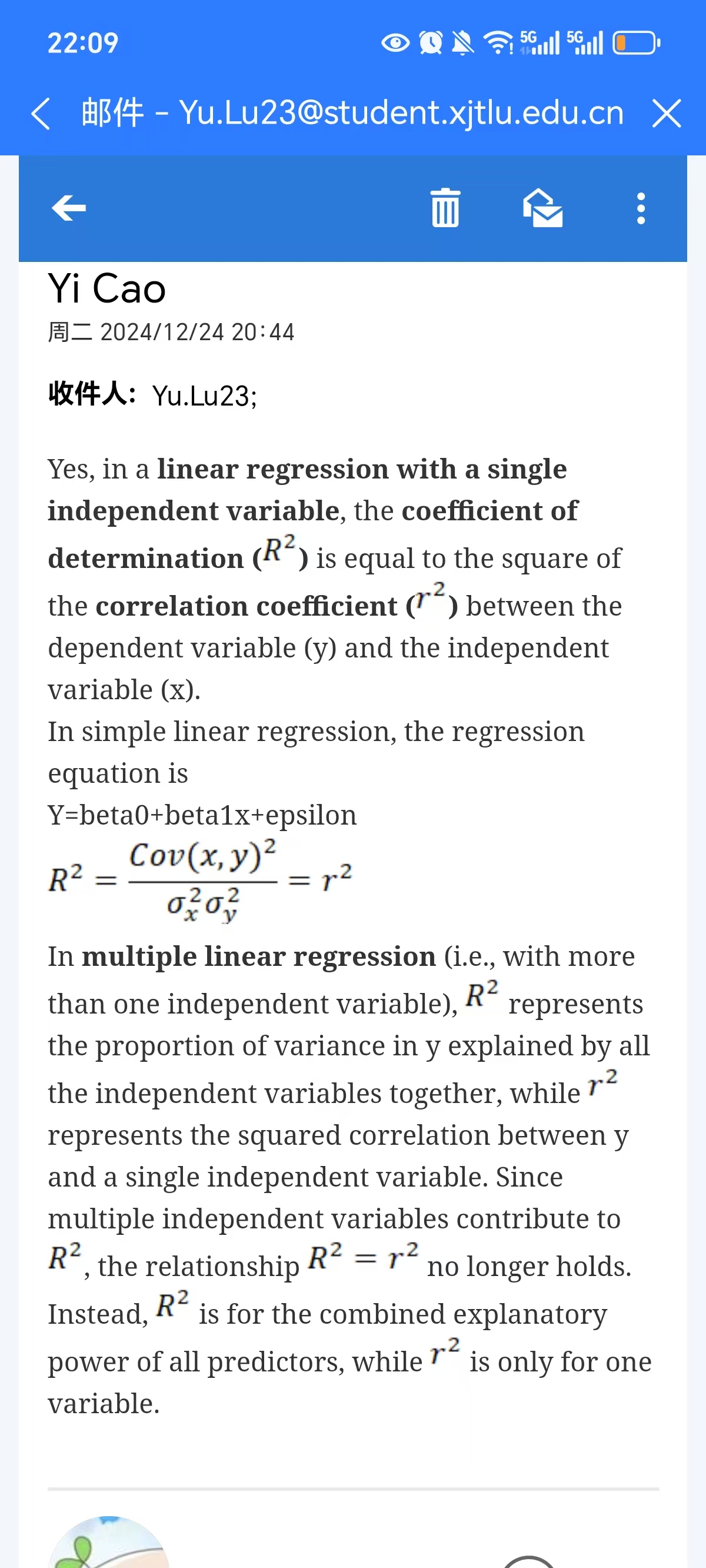
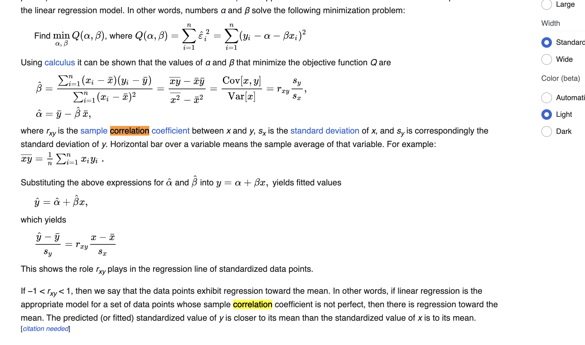
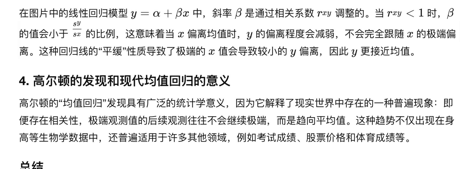


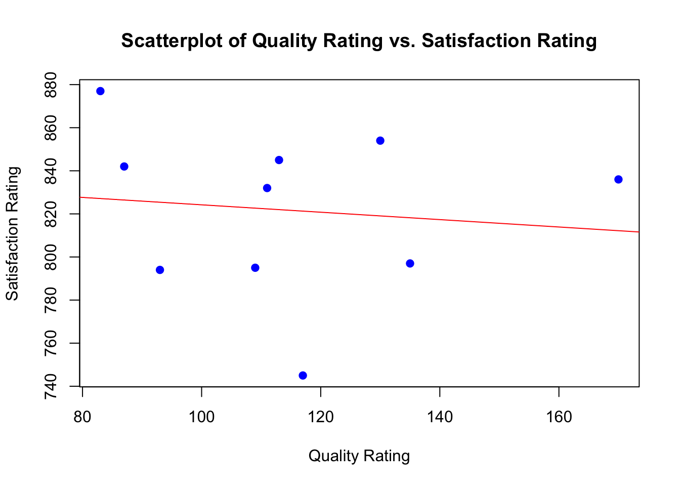

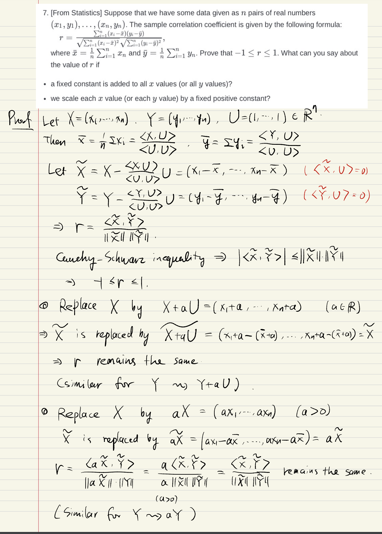
 inferences from 2 samples introduces the differences between two populaton means using matched pairs but correlaition and regression analyze the association between the 2 variables and if such an association exists we wnat to describe it with an equation that can be used for predictions