Calculus and Multivariable Calculus

surface and volume of Steinmetz solid

( See the attached vedio for further explanation: http://youtube.com/watch?v=Vf0nqYaLWIs )

Professor. Wang Duo, a very charismatic and responsible Calculus teacher who has worked for our country in the area of math for at least 50 years (which was his target before and he has realized his dream!), always says “You should try to solve one problem many times with new methods to handle and understand knowledge better”

For math learning, focusing too much on exams is not so meaningful. We should experience its beauty from the bottom of our hearts. I did not reach my target in the Multivariable Calculus and the Linear Algebra models, but Dr. Bohuan Lin said:“Exams (especially written exams) require one to figure out solutions within a very short time period, and moreover, under an intense atmosphere. From my point of view, it is really not a problem if one fails to solve those difficult and nonstandard problems under such a condition. Of course, for math study (so as for the study of other things), we should not be satisfied with merely being able to solve”standard problems”, but just try to challenge and improve yourself with deep/difficult questions under a daily condition with a natural mood, since this is the common situation in which you will be working on various tasks in your future career. ”

There are many ways to solve problems, and all of them are interesting when multiple integrals occur.

2 cylinders

It is easy

surface

volume

use method of sections directly

3 cylinders

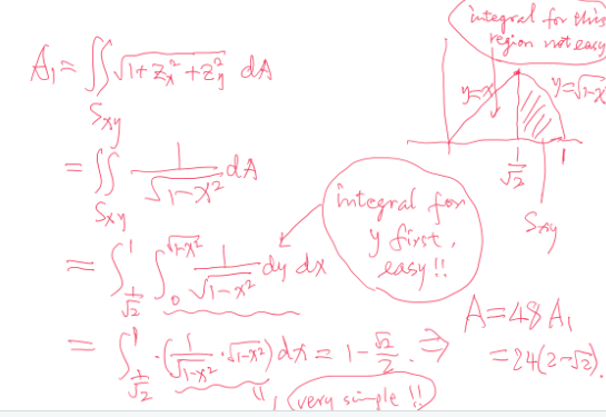
surface

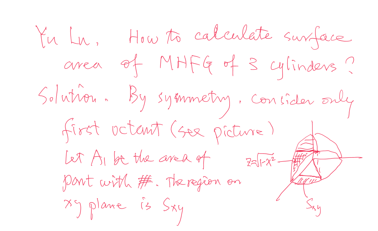
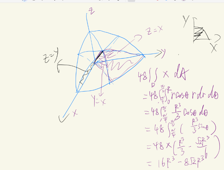
see the photo attached, which is the easiest way for computation:

volume

method 1—do not draw it(using conditional inferences)

Thanks to Dr.Bohuan Lin to teach me such a clever way which we do not need to draw the picture(only use conditional equations to solve it is interesting and a little difficult to handle it correctly).

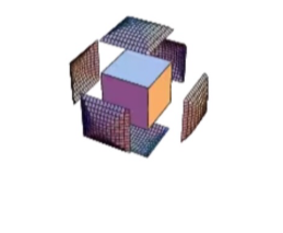
The picture behind the method is attached to “Steinmetz(mou he fang gai)’s photo behind.png”

We have the set ( D ) defined as: \[ D \triangleq \left\{(x, y, z) \mid \begin{cases} x^2 + y^2 \leq 4 \\ y^2 + z^2 \leq 4 \\ z^2 + x^2 \leq 4 \end{cases} \right\} \]

From \[x^2+ y^2 \leq 4 , x^2 + z^2 \leq 4 \] we derive: if \[ |x| \geq \sqrt{2},|y| \leq \sqrt{2} \quad \text{then} \quad |z| \leq \sqrt{2} \] (and < is the same shape)

Similarly:

if \[|z| \geq \sqrt{2} ,|x| \leq \sqrt{2} \quad \text{then} \quad |y| \leq \sqrt{2} \]

And: if \[ |z| \geq \sqrt{2},|y| \leq \sqrt{2} \quad \text{then} \quad |x| \leq \sqrt{2} \] Therefore: \[ D = D_{\leq \sqrt{2}} \cup \bar{D} \]

Where: \[ D_{\leq \sqrt{2}} = \left\{(x, y, z) \in D \mid |x|, |y|, |z| \leq \sqrt{2} \right\} \] \[ \begin{aligned} &= \left\{ (x, y, z) \in \mathbb{R}^3 \mid |x|, |y|, |z| \leq \sqrt{2} \right\} \\ &= [-\sqrt{2}, \sqrt{2}] \times [-\sqrt{2}, \sqrt{2}] \times [-\sqrt{2}, \sqrt{2}] \end{aligned} \]

And: \[ \bar{D} = \left\{(x, y, z) \in D \mid |x|, |y|, |z| > \sqrt{2} \right\} \]

Thus: \[ \bar{D} = \bar{D}_{|x| > \sqrt{2}} \cup \bar{D}_{|y| > \sqrt{2}} \cup \bar{D}_{|z| > \sqrt{2}} \]

(This also implies: \[ D_{\leq \sqrt{2}} = \left\{(x, y, z) \in D \mid |x|, |y|, |z| \leq \sqrt{2} \right\} \])

We derive: \[ \bar{D} = \left\{ (x, y, z) \mid |x| > \sqrt{2} \right\} \cup \left\{ (x, y, z) \mid |y| > \sqrt{2} \right\} \cup \left\{ (x, y, z) \mid |z| > \sqrt{2} \right\} \]

Thus, combining all components, we get: \[ D = \left( D_{\leq \sqrt{2}} \cup \bar{D}_{|x| > \sqrt{2}} \cup \bar{D}_{|y| > \sqrt{2}} \cup \bar{D}_{|z| > \sqrt{2}} \right) \] So we could decompose it into a cube in the center and 6 common volume. the 6 volume: 6 \(\int_{ \sqrt{2}}^{2}4(4-x^2) dx\)

In summary, the whole volume is \((2 \sqrt 2)^3 +6\int_{ \sqrt{2}}^{2}4(4-x^2) dx\)

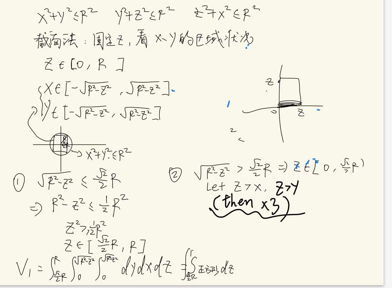
method 2—cross-section method

Thanks to Dr. Haoran Chen for teaching us such method.

We suppose z>x, z>y,（then *3） then we could continue decompose it into (1)z~(\(\sqrt 2\),2) and (2)z~(\(0,\sqrt 2\))(based on whether the square is out of the circle)

method 3

see the photo attached

(sequence)sinx/x’s 0-infinite’s integral

Dr.Fajin Wei teach me how to do it. He is very good at Calculus and Modeling. He is kind to help our students. Thanks to him very much!

integral problems with solution of alternating integral test

question: does \[\int_{0}^{\infty}sinx/x\,dx\] converge?

It is easy to think of these 2 famous but difficultly proved formula: \[\int_{-\infty}^{\infty}sinx/x\,dx=\pi \] \[\int_{-\infty}^{\infty}e^{-x^2}\,dx=\pi \] However, they are not useful, which is how charasmatic the math is! I love math!

\[=\Sigma_{n=1}^{\infty}\int_{2(n-1)\pi}^{2n\pi}sinx/x\,dx \] Then we let \(x-[2(n-1)\pi]=y\)(dx=dy)

so \[=\Sigma_{n=1}^{\infty}\int_{0}^{2\pi}siny/(y+[2(n-1)\pi])\,dy\] =\[=\Sigma_{n=1}^{\infty}\int_{0}^{\pi}siny/(y+[2(n-1)\pi])\,dy+\Sigma_{n=1}^{\infty}\int_{\pi}^{2\pi}siny/(y+[2(n-1)\pi])\,dy\]

Then we let y-\(\pi\)=z(dy=dz)

\[=\Sigma_{n=1}^{\infty}\int_{0}^{\pi}siny/(y+[2(n-1)\pi])\,dy+\Sigma_{n=1}^{\infty}\int_{0}^{\pi}-sinz/(z+[(2n-1)\pi])\,dz\] \[=\Sigma_{n=1}^{\infty}\int_{0}^{\pi}sinm/(m+[2(n-1)\pi])\,dm+\Sigma_{n=1}^{\infty}\int_{0}^{\pi}-sinm/(m+[(2n-1)\pi])\,dm\]

so if \[a_n=\int_{0}^{\pi}sinm/(m+(n-1)\pi)\] \[\int_{0}^{\infty}sinx/x\,dx=a_1-a_2+a_3-a_4+...+a_n\], which is an alternating series!

Coincidently, it is decresing and \(a_n<\int_{0}^{\pi}1/(n-1)\pi\,dm=1/(n-1)\), and \(\lim_{{n \to \infty}} \left( \frac{1}{n-1} \right) = 0\) so \(\lim_{{n \to \infty}}a_n=0\) So it converges(Alternating series test).

similar question 2

Thanks for Dr.Chi-Kun Lin to teach me this kind of problems!

\[ \int_0^\infty \frac{1}{1 + x^p \sin^2 x} \, dx \]

\[ \sum_{n=0}^\infty \int_0^{\frac{\pi}{2}} \frac{1}{1 + \left( n + \frac{1}{2} \right)^2 p \sin^2 t} \, dt = \int_0^{\frac{\pi}{2}} \frac{1}{1 + \left( n + \frac{1}{2} \right)^2 p \sin^2 t} \, dt \]

\[\Sigma\int_0^{\frac{\pi}{2}} \frac{1}{1 + \left( n\pi/2 + t \right)^ p \sin^2 t} \, dt + \int_0^{\frac{\pi}{2}} \frac{1}{1 + \left(( n + 1 \right)\pi/2-t)^ p sin^2t} \, dt\]

for:

\[ x_n = \Sigma\int_0^{\frac{\pi}{2}} \frac{1}{1 + \left( n\pi/2 + t \right)^ p \sin^2 t} \, dt + \int_0^{\frac{\pi}{2}} \frac{1}{1 + \left(( n + 1 \right)\pi/2-t)^ p sin^2t} \, dt, \]

there has

\[2 \int_0^{\frac{\pi}{2}} \frac{1}{1 + \left( (n + 1) \frac{\pi}{2} \right)^ p t^2} \, dt \leq x_n \leq 2 \int_0^{\frac{\pi}{2}} \frac{1}{1 + \left( (n + 1) \frac{\pi}{2} \right) ^p \frac{4}{\pi^2} t^2} \, dt\]

3. However, the integrals on both sides of the inequality can be calculated separately. For example:

\[ \int_0^1 \frac{1}{1 + \left( (n + 1) \frac{\pi}{2} \right)^ p t^2} \, dt = \frac{1}{\sqrt{((n + 1) \frac{\pi}{2} )^p}} \arctan \left( \sqrt{(n + 1) \frac{\pi}{2}}^{2p}\pi/2 \right) \geq \frac{1}{\sqrt{(n + 1) \frac{\pi}{2} }^{2p} } \frac{\pi}{4} \]

Extreme Values of Function using not only Lagrange but the same philosophy

introduction with the relationship between it and lasso

The Lagrange multiplier method can transform constrained problems into unconstrained problems, which is a great wisdom. It can be used to solve lasso, and lasso is an interesting and wonderful method for dimensionality reduction in statistics, which makes me feel that the journey of learning multivariate calculus is a joy：

Lagrange Multipliers Perspective of Penalized Models

Lagrange multipliers provide a way to incorporate constraints into optimization problems. In the context of penalized regression, we can view the regularization term as a constraint on the size of the coefficients.

Choose Lasoo as an example, the Lagrange multipliers perspective could be expressed as:

\[ \left( \hat{\alpha}, \hat{\beta} \right) = \arg \min \left\{ \sum_{i=1}^{N} \left( y_{i} - \alpha - \sum_{j} \beta_{j} x_{ij} \right)^{2} \right\} \quad \text{subject to} \quad \sum_{j} \left| \beta_{j} \right| \leq t. \]

i.e.

\[ g(\beta)= \sum_{j} \left| \beta_{j} \right| - t \leq 0 \]

\[ L(\alpha,\beta, \lambda) = \sum_{i=1}^{N} \left( y_{i} - \alpha - \sum_{j} \beta_{j} x_{ij} \right)^{2} + \lambda \left( \sum_{j} \left| \beta_{j} \right| - t \right) \]

\[ \partial L / \partial \alpha = 0 \]

\[ \hat{\alpha} = \bar{y} - \sum_{j} \hat{\beta}_{j} \bar{x}_{j} \]

\[ \partial L / \partial \beta_{j} = 0 \]

\[ -2 \sum_{i=1}^{N} x_{ij} \left( y_{i} - \hat{\alpha} - \sum_{k} \hat{\beta}_{k} x_{ik} \right) + \lambda \cdot sign(\hat{\beta}_{j}) = 0 \]

This may use the iterative method to solve the equation.

Generally, the formula could be expressed as:

\[ \min_{\beta} \left\{ \lVert y - X\beta \rVert_2^2 + \lambda \lVert \beta \rVert_p^p \right\} \]

where \(\lVert \beta \rVert_p^p\) is the \(L^p\) norm of the coefficients, which serves as a penalty term.

The gradient of the objective function of Ridge with respect to \(\beta\) is given by:

\[ \nabla J(\beta) = -2X^T(y - X\beta) + \lambda \nabla \lVert \beta \rVert_p^p \]

(see matrix form (Go to Matrix Form) below for more details)

This should be set to zero to find the optimal \(\beta\), which means the gradient of the loss function (the first term) is equal to the gradient of the penalty term (the second term) scaled by \(\lambda\).

Geometric Interpretation of Penalized Models in Lagrange Multipliers Perspective

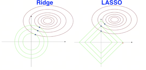
Summary

• Lasso Regression uses L1 regularization to achieve feature selection, and its optimization problem can be transformed into a constrained optimization problem.
• Lagrange Multipliers provide a method to handle constraints in optimization problems by converting them into unconstrained problems and introducing multipliers to adjust the regularization strength.

In Lasso regression, the L1 regularization constraint can be handled using Lagrange multipliers, converting the problem into one with multipliers that adjust the strength of regularization. ### Problem

Find extreme values of

\[ f(x, y) = \cos x + \cos y + \cos (x + y). \]

Solution

Since cosine is a periodic function, we can consider the region ( 0 x ), ( 0 y ) (bounded and closed region) to find the maximal and minimal values.

Firstly, we consider the interior of the region to find stationary points:

\[ f_x = -\sin x - \sin (x + y) = 0 \] \[ f_y = -\sin y - \sin (x + y) = 0 \]

This implies:

\[ \sin x = \sin y \]

Then, inside the region (not on boundary), we have three cases:

1. ( y = x )
2. ( y = - x ) for ( 0 < x < )
3. ( y = 3- x ) for ( < x < 2)

Case 1

\[ \sin x + \sin (x + y) = \sin x + 2 \sin x \cos x = 0 \] \[ \sin x (2 \cos x + 1) = 0 \]

This implies:

\[ x = \pi, y = \pi \] or \[ x = \frac{2\pi}{3}, y = \frac{2\pi}{3} \] or \[ x = \frac{4\pi}{3}, y = \frac{4\pi}{3} \]

Evaluating the function at these points:

\[ f(\pi, \pi) = -1 \] \[ f\left( \frac{2\pi}{3}, \frac{2\pi}{3} \right) = -\frac{3}{2} \] \[ f\left( \frac{4\pi}{3}, \frac{4\pi}{3} \right) = -\frac{3}{2} \]

Case 2

\[ \sin x + \sin (x + y) = \sin x + \sin \pi = \sin x = 0 \]

This implies:

\[ x = \pi, y = 0 \] (on boundary)

Case 3

\[ \sin x + \sin (3\pi - x) = \sin x = 0 \]

This implies:

\[ x = \pi, y = 2\pi \] (also on boundary)

On the Boundary

Due to periodic property, we consider:

\[ x = 0, 0 \leq y \leq 2\pi \] and \[ y = 0, 0 \leq x \leq 2\pi \]

Evaluating the function at these boundaries:

\[ f(0, y) = 1 + 2 \cos y, \min = -1, \max = 3 \] \[ f(x, 0) = 1 + 2 \cos x, \min = -1, \max = 3 \]

So,

\[ \max f(x, y) = 3 \text{ at } (2n\pi, 2k\pi) \text{ for any } n, k \in \mathbb{Z} \] \[ \min f(x, y) = -\frac{3}{2} \text{ at } \left( (2n+1)\pi \pm \frac{\pi}{3}, (2k+1)\pi \pm \frac{\pi}{3} \right) \]

one application problem about directional derivative and gradient

Thanks to Boyun Pang to let me know this interesting question and thanks to Dr. Wang to teach me such clever method. The temperature ( T ) in degrees Celsius at ((x, y, z)) is given by

\(T = \frac{10}{{x^2 + y^2 + z^2}}\)

where distances are in meters. A bee is flying away from the hot spot at the origin on a spiral path so that its position vector at time ( t ) seconds is \(\mathbf{r}(t) = t \cos(\pi t) \mathbf{i} + t \sin(\pi t) \mathbf{j} + t \mathbf{k}\)

Determine the rate of change of ( T ) in each case:

1. With respect to distance traveled at time ( t=1 ).
2. With respect to time at ( t = 1 ).

(Think of two ways to do this.)

\[ \frac{dT}{dS} = \nabla f \cdot \mathbf{R}'(S) \]

\[ \frac{dT}{dS} = f_x \cdot x'(S) + f_y \cdot y'(S) + f_z \cdot z'(S) \]

\[ ||\vec{r(t)}||=\int_{0}^{t} \sqrt{x'^2 + y'^2 + z'^2} \, dt = S(t) \]

\[ \mathbf{r}(t(S)) = \mathbf{R}(S) \]

\[ \vec{R(S)}' =\mathbf{r}(t(S)) \mathbf{t}(S)=\mathbf{r}(t(S))\frac{1}{\mathbf{S}(t)}(inverse function) =\frac{\mathbf{r}’(t)}{||\mathbf{r}’(t)||} \]

\[ \mathbf{R}'(S) = \frac{\mathbf{r}'(t(S)) \cdot t'(S)}{\sqrt{x'^2 + y'^2 + z'^2}} \]

\[ \mathbf{R}(t) = \mathbf{r}(t) \]

remark of Derivative

\(y'=\frac{d}{dx}\cdot y\)

\(y''=\frac{d}{dx} \frac{d}{dx}\cdot y\)=\(\frac{d^2y}{dx^2}\cdot y\)