APH203

Lecture 1

6 examples of Time Series Data

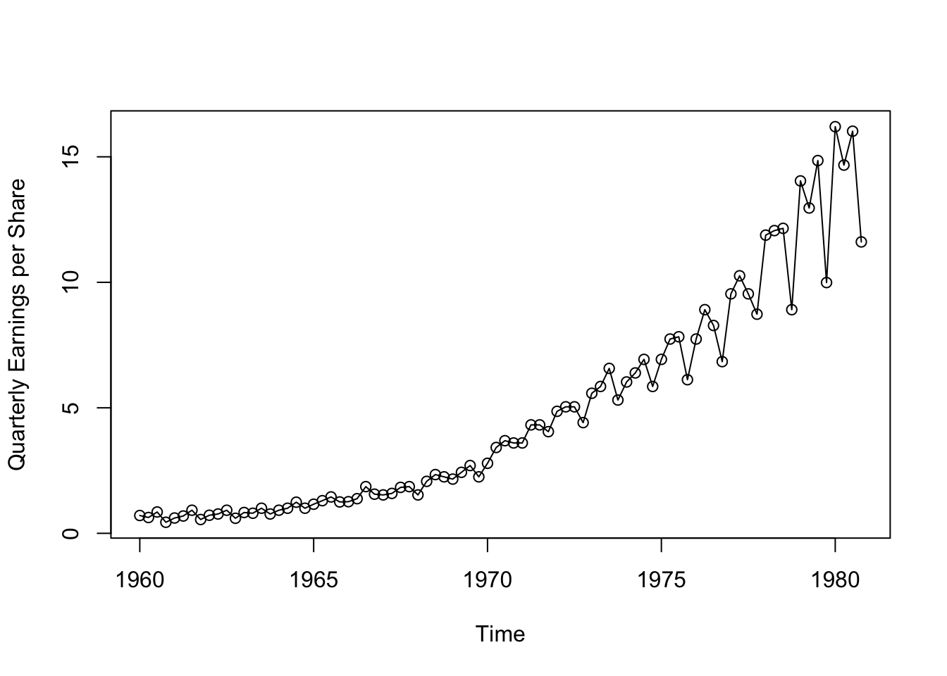
library(astsa)
plot(jj,type="o",ylab="Quarterly Earnings per Share")

plot(gtemp_both,type="o",ylab="Global Temperature Deviations")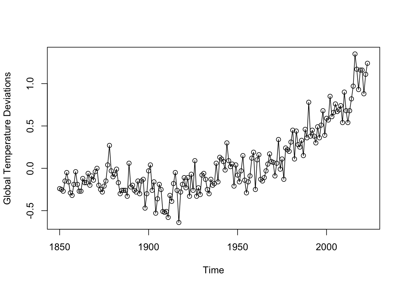

library(astsa)
library(xts)

Loading required package: zoo

Attaching package: 'zoo'

The following objects are masked from 'package:base':

    as.Date, as.Date.numeric

djiar = diff(log(djia$Close))[-1]
plot(djiar,ylab="DJIAReturns",type="n")

lines(djiar)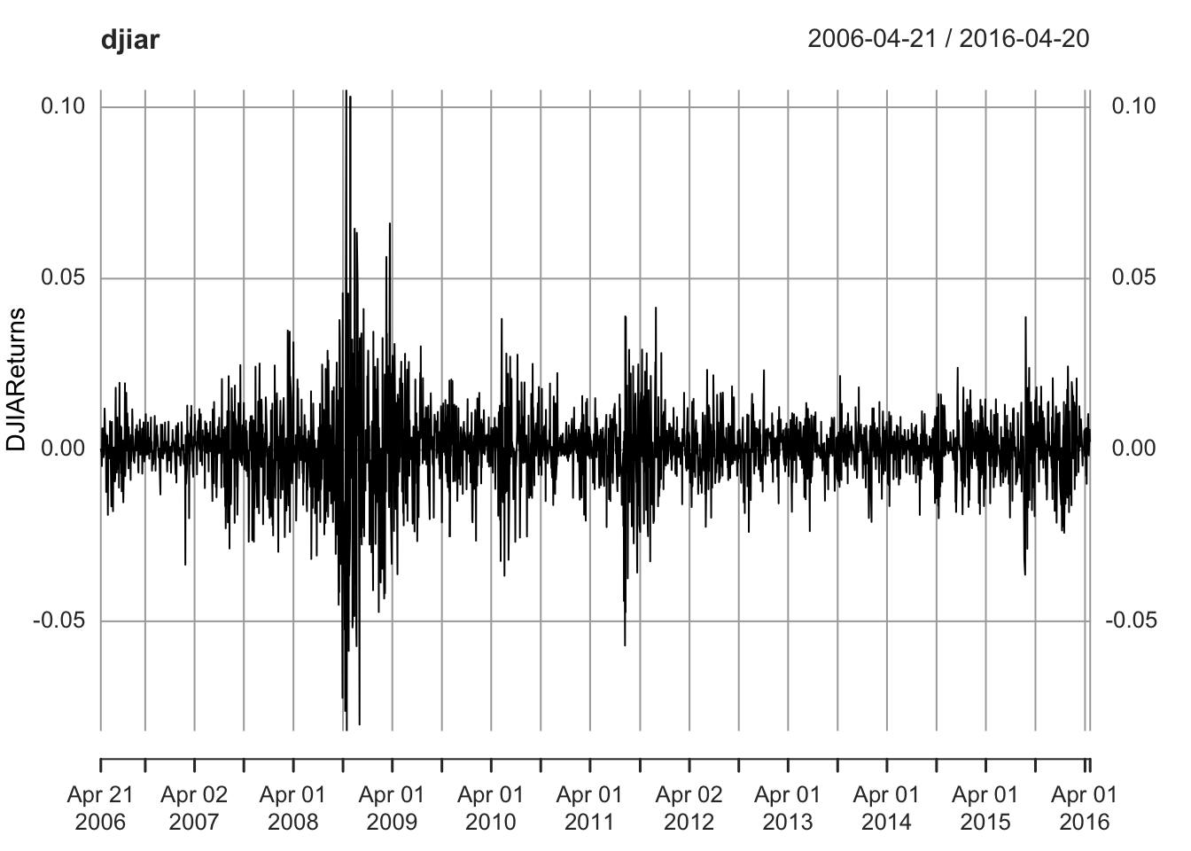

return: 投资回报率

Lesson: Leave quickly once get some profit

par(mfrow =c(2,1))
plot(soi, ylab="", xlab="", main="Southern Oscillation Index")
plot(rec, ylab="", xlab="", main="Recruitment")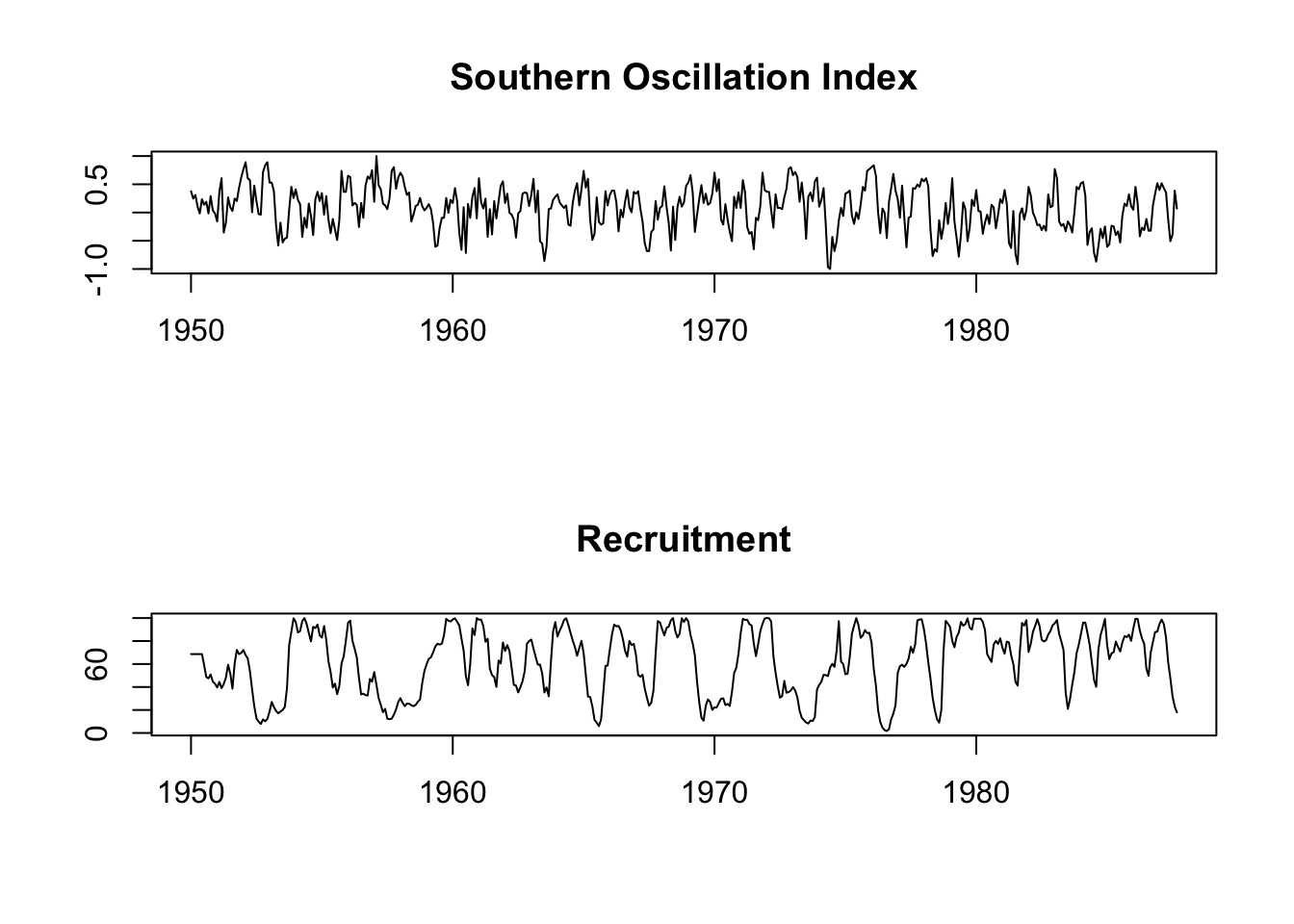

par(mfrow=c(2,1))
ts.plot(fmri1[,2:5], col=1:4, ylab="BOLD", main="Cortex")
ts.plot(fmri1[,6:9], col=1:4, ylab="BOLD", main="Thalamus & Cerebellum")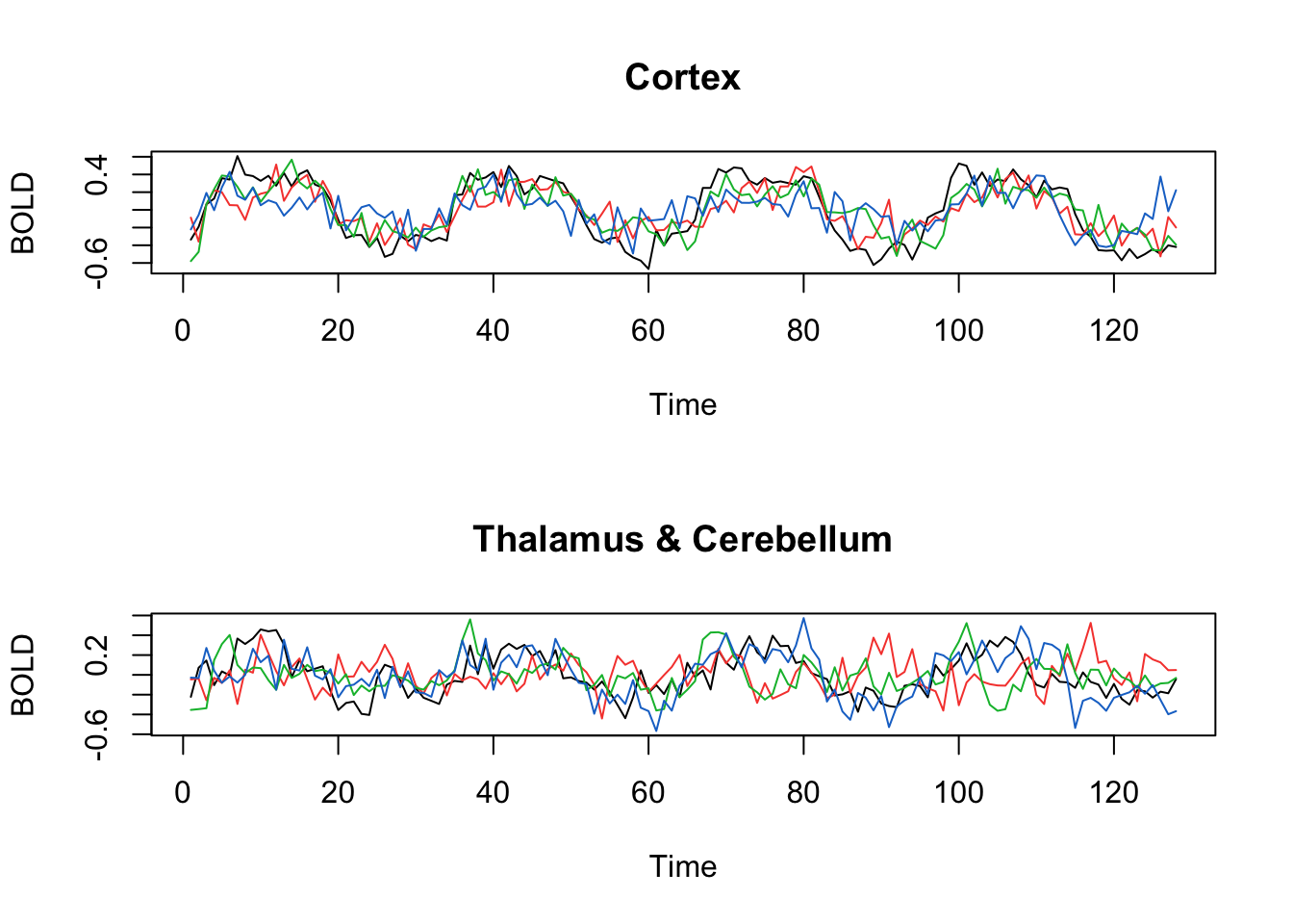

periodic

# Earthquakes and Explosions
par(mfrow=c(2,1))
plot(EQ5, main="Earthquake")
plot(EXP6, main="Explosion")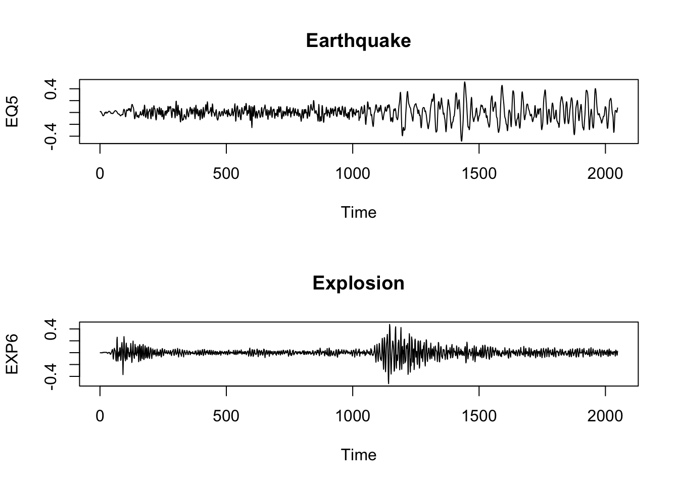

classification of Time Series Data

• Univariate vs Multivariate

• Continuous vs Discrete

• Stationary vs Non-Stationary

• Linear vs Non-Linear

Methods for Time Series Analysis

• Descriptive Methods

• Statistical Time Series Analysis

• White noise

w = rnorm(500,0,1) # 500 N(0,1) variates
plot.ts(w, main="white noise")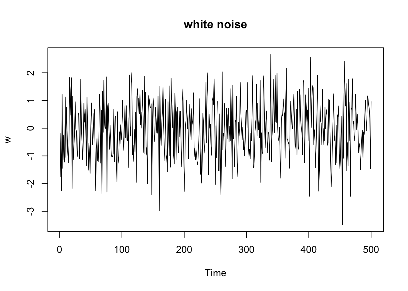

• Moving Average and Filtering

\(v_t = \frac{1}{3}(w_{t-1}+w_t+w_{t+1})\)

v = filter(w, sides=2, filter=rep(1/3,3)) # moving average 
plot.ts(v, ylim=c(-3,3), main="moving average")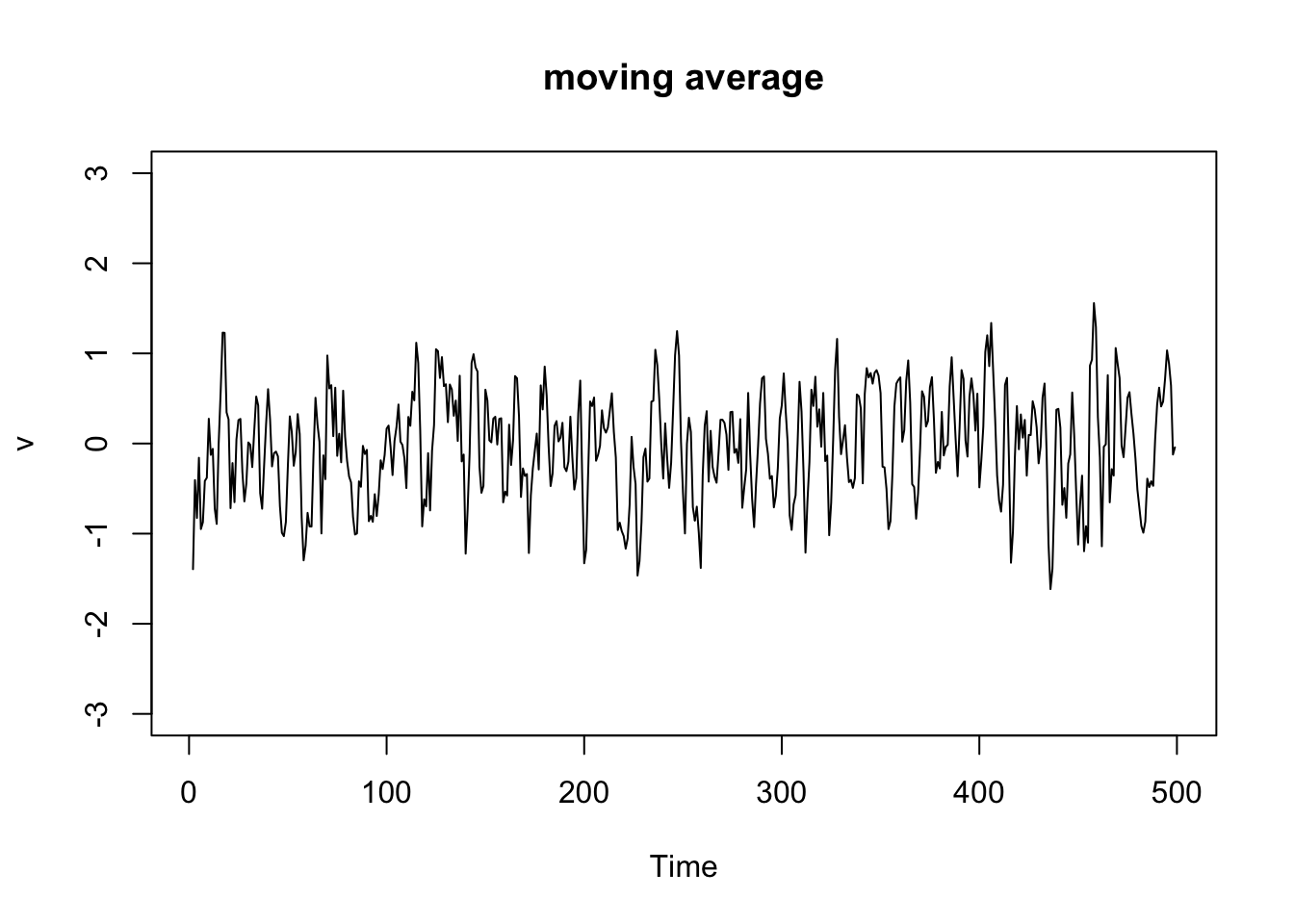

new model after 1970’s ARIMA

Since the Gaussian-Markov assumption (\(E(\epsilon) =0\) and \(\epsilon \sim N\) i.i.d )is so strict, and heteroscedasticity is often observed in the real data, new models were developed after 1970’s.

?Questions: If the variance ….. why not WLS?

Basic background knowledge (review of the past)

proof of the Chebyshev’s Inequality

• Proof of the Markov’s Inequality

If \(X\) is a non-negative random variable and \(a>0\), then \[P(X\ge a) \le \frac{E(X)}{a}\] \[ E(X) = \int_{0}^{\infty} x f(x) \, dx \]

\[ E(X) = \int_{0}^{a} x f(x) \, dx + \int_{a}^{\infty} x f(x) \, dx \] \[ \int_{a}^{\infty} x f(x) \, dx \geq \int_{a}^{\infty} a f(x) \, dx = a \int_{a}^{\infty} f(x) \, dx \]

\[ E(X) \geq a \cdot P(X \geq a) \]

\[ P(X \geq a) \leq \frac{E(X)}{a} \]

• Proof of the Chebyshev’s Inequality

\[ P((X - \mu)^2 \geq k^2\sigma^2) \leq \frac{E[(X-\mu)^2]}{k^2\sigma^2}=\frac{\sigma^2}{k^2\sigma^2} = \frac{1}{k^2} \]

\[ P(|X - \mu| \geq k\sigma) \leq \frac{1}{k^2} \]

Law of Large Numbers (LLN)

• Weak Law of Large Numbers

Let \(X_1, X_2, \ldots, X_n\) be a sequence of i.i.d. random variables with finite mean \(\mu\) and finite variance \(\sigma^2\). Then for any \(\epsilon > 0\),

\[ P\left(\left|\frac{1}{n}\sum_{i=1}^{n} X_i - \mu\right| \geq \epsilon\right) \to 0 \text{ as } n \to \infty \]

• Strong Law of Large Numbers

Let \(X_1, X_2, \ldots, X_n\) be a sequence of i.i.d. random variables with finite mean \(\mu\). Then,

\[ P\left(\lim_{n \to \infty} \frac{1}{n}\sum_{i=1}^{n} X_i = \mu\right) = 1 \]

• Proof of the Weak Law of Large Numbers

By Chebyshev’s inequality, for any \(\epsilon > 0\),

\[ P\left(\left|\frac{1}{n}\sum_{i=1}^{n} X_i - \mu\right| \geq \epsilon\right) \leq \frac{\text{Var}\left(\frac{1}{n}\sum_{i=1}^{n} X_i\right)}{\epsilon^2} = \frac{\frac{1}{n^2}\cdot n\sigma^2}{\epsilon^2}=\frac{\sigma^2/n}{\epsilon^2} = \frac{\sigma^2}{n\epsilon^2} \]

As \(n \to \infty\), \(\frac{\sigma^2}{n\epsilon^2} \to 0\). Therefore, \[ P\left(\left|\frac{1}{n}\sum_{i=1}^{n} X_i - \mu\right| \geq \epsilon\right) \to 0 \text{ as } n \to \infty \]

• Proof of the Strong Law of Large Numbers (using Borel-Cantelli Lemma)

By Chebyshev’s inequality, for any \(\epsilon > 0\),

\[ P\left(\left|\frac{1}{n}\sum_{i=1}^{n} X_i - \mu\right| \geq \epsilon\right) \leq \frac{\sigma^2}{n\epsilon^2} \]

Let \(A_n = \left\{\left|\frac{1}{n}\sum_{i=1}^{n} X_i - \mu\right| \geq \epsilon\right\}\). Then,

\[ \sum_{n=1}^{\infty} P(A_n) \leq \sum_{n=1}^{\infty} \frac{\sigma^2}{n\epsilon^2} = \frac{\sigma^2}{\epsilon^2} \sum_{n=1}^{\infty} \frac{1}{n} \]

The series \(\sum_{n=1}^{\infty} \frac{1}{n}\) diverges, so we cannot directly apply the Borel-Cantelli lemma here. However, we can use a modified approach. Consider the events \(B_k = \left\{\left|\frac{1}{2^k}\sum_{i=1}^{2^k} X_i - \mu\right| \geq \epsilon\right\}\). Then,

\[ \sum_{k=1}^{\infty} P(B_k) \leq \sum_{k=1}^{\infty} \frac{\sigma^2}{2^k\epsilon^2} = \frac{\sigma^2}{\epsilon^2} \sum_{k=1}^{\infty} \frac{1}{2^k} = \frac{\sigma^2}{\epsilon^2} \]

Since \(\sum_{k=1}^{\infty} P(B_k)\) converges, by the Borel-Cantelli lemma(如果一系列独立事件的概率之和是有限的，那么这些事件无限次发生的概率为零), we have

\[ P(B_k \text{ i.o.}) = 0 \]

(i.o means infinitely often)

(p.s.: if 一系列独立事件的概率之和是无限的，并且这些事件是独立的，那么这些事件无限次发生的概率为一)

This implies that \[ P\left(\lim_{k \to \infty} \frac{1}{2^k}\sum_{i=1}^{2^k} X_i = \mu\right) = 1 \]

Now, for any \(n\), there exists a \(k\) such that \(2^k \leq n < 2^{k+1}\). We can write \[ \frac{1}{n}\sum_{i=1}^{n} X_i = \frac{1}{n}\left(\sum_{i=1}^{2^k} X_i + \sum_{i=2^k+1}^{n} X_i\right) \]

As \(k \to \infty\), the second term \(\frac{1}{n}\sum_{i=2^k+1}^{n} X_i\) becomes negligible, and we have \[ \lim_{n \to \infty} \frac{1}{n}\sum_{i=1}^{n} X_i = \mu \]

with probability 1. Therefore,

\[ P\left(\lim_{n \to \infty} \frac{1}{n}\sum_{i=1}^{n} X_i = \mu\right) = 1 \]

Central Limit Theorem (CLT)

Lecture 3

AIC and BIC

KL (Kullback-Leibler) divergence

• defination of the entropy

The entropy of a discrete random variable \(X\) with probability mass function \(P(X)\) is defined as:

\[ H(X) = -\sum_{x} P(x) \log(P(x)) \]

• Definition of KL divergence

The Kullback-Leibler (KL) divergence is a measure of how one probability distribution diverges from a second, expected probability distribution. It is defined as follows:

For discrete probability distributions \(P\) and \(Q\) defined on the same probability space, the KL divergence from \(Q\) to \(P\) is given by:

\[ D_{KL}(P || Q) = \sum_{x} P(x) \log\left(\frac{P(x)}{Q(x)}\right)=\sum_x P(x) \frac{1}{\log(Q(x))} - \sum_x P(x) \frac{1}{\log(P(x))}\\ = H(P,Q) -H(P) \] P(x) is the true distribution, Q(x) is the approximating distribution (proposed p.d.f)

For continuous probability distributions, the KL divergence is defined as:

\[ D_{KL}(P || Q) = \int_{-\infty}^{\infty} p(x) \log\left(\frac{p(x)}{q(x)}\right) dx \]

where \(p(x)\) and \(q(x)\) are the probability density functions of \(P\) and \(Q\), respectively.

• example

• disadvantage: we do not the true distribution P(x)

AIC (Akaike Information Criterion)

By Akaike (1974), although the true distribution \(P(x)\) is unknown, we can use the maximum likelihood estimate (MLE) to approximate it. The AIC is derived from an estimate of the KL divergence between the true model and a candidate model.

AIC is defined as:

\[ AIC = -2 \log(L) + 2k \]

AICc

AICc is a corrected version of AIC that adjusts for small sample sizes. It is defined as:

\[ AICc = AIC + \frac{2k(k+1)}{n-k-1} \]

when n goes to infinity, AICc converges to AIC.

BIC (Bayesian Information Criterion)

• Bayesian Thm

\[ P(A|B) = \frac{P(B|A)P(A)}{P(B)} \]

A goes to \(\theta\), B goes to x

\[ \hat \theta = \arg\max_{\theta} P(\theta|x) = \arg\max_{\theta} \frac{P(x|\theta)P(\theta)}{P(x)} = \arg\max_{\theta} P(x|\theta)P(\theta) \]

• BIC formula

\[ BIC = -2 \log(L) + k \log(n) \]

loglikelihood penalized by the number of parameters and the sample size

loglikelihood could be replaced by the loss function

BIC is more popular used in high-dimensional data analysis. If not in high-dimensional data analysis, AIC and BIC values are similar.

reference

https://harvard-iacs.github.io/2018-CS109A/a-sections/a-section-2/presentation/a-sec2-MLEtoAIC.pdf

Emphasis

stationary

non-parametric

$x_1,

eg.

\(e^x = \sum_{n=0}^{\infty} \frac{x^n}{n!}\) 多项式逼近

B-spline

Kernel

非参–也有不好的方面

拿到数据，想要估计，选择哪个kernel function都可以，只是估计效率的问题，结果差不多，尤其是对于小样本