Linear Regression

Partial modeling–P(x|y)

For many points, there are many possible regression functions f (nonparametric) so it is useful to restrict to simple functions described by a few parameters.

Though true regression functions are never linear, we assume the dependence of Y on $X_1$…$X_n$ is linear.

regression function: x—-> f(x) : $$ E[Y

X=x]= \int yh(y

x)dy$(ps: the conditional median:m(x)$\int_{-\infty}^{m(x)}\ h(y

x)dy=1/2$$)

Simple linear regression

OLS(Ordinary Least-Squares): Historically, the OLS method was introduced before the systematic understanding of conditional expectation. The OLS method was proposed by French mathematician Adrien-Marie Legendre in 1805 and later developed by Carl Friedrich Gauss in 1809. The OLS method was created to find the regression coefficients that best fit the data. An interesting geometry explaination in Linear Algebra’s projection matrix of OLS in multiple(simple) linear regression:
Conditional Expectation: After the OLS method was established, it was recognized that the regression equation obtained through OLS is actually the expected value of (Y) given (X), i.e., the conditional expectation (E(Y|X=x)). Under the classical linear regression assumptions, the OLS estimate is an unbiased estimate of the conditional expectation.

Specifically, for a simple linear regression model ($Y = \beta_0 + \beta_1X + \epsilon$):

OLS Estimate: Through the OLS method, we obtain the estimated regression coefficients ($\hat{\beta}_0$) and ($\hat{\beta}_1$), thus writing the regression equation ($\hat{Y} = \hat{\beta}_0 + \hat{\beta}_1X$). (based on the smallest RSS)
Conditional Expectation: According to the model assumption, the conditional expectation (E(Y|X=x)) should be ($\beta_0 + \beta_1x$)(which is called the real regression line(not the true line) and could not be seen in practice). The regression equation obtained through OLS, ($\hat{Y} = \hat{\beta}_0 + \hat{\beta}_1X$), is an estimate of (E(Y|X=x)).

In summary, OLS(similar to MLE in SLR) is the best way to estimate the true model, which generates the unbiased estimators of the real regression line that based on $E[y_i

x]$.

Another explaination–analogy of population mean in sampling distribution:

essence of SLR relavant to ρ (correlation coefficient)

\[\hat{y}-\bar{y}/sd(\hat{y})=\rho(\hat{x}-\bar{x}/sd(\hat{x}))\]

Proof using covariance when it is normal distribution(Teacher:shisong mao)

Hypothesis test in (simple/multiple–the same philosophy) Linear Regression

t-statistics for estimators

z—-t—-F

slope

$H_0$:$\beta_1$=0 ###### t for testing significance of regression Because $y_i=\hat{\beta}_0+\hat{\beta}_1 x_i$~NID($\beta_0+\beta_1x_i,\sigma^2$), $\beta_1$~N($\beta_1$,$\sigma^2\Sigma (x_i-\bar{x})^2$ so if $\sigma$ is known, $\hat{\beta}_1/ \sqrt {\sigma^2/\Sigma (x_i-\bar{x})^2}$ but if $\sigma$ is unknown, $t_0=\hat{\beta}_1/se( \hat{\beta}_1)$, which just substitute $\sigma$’s unbiased estimation($\Sigma (y_i-\hat{y})^2/n-2$, which is RSS)for $\sigma$.

F of analysis of variance for testing the significance of regression(2 ways to understand F test—model interpretation and hypothesis test with noncentralirity parameter(0 or not 0)

\[\frac{\Sigma (y_i-\hat{y})^2}{\sigma^2p}/\frac{\Sigma(\hat{y}-\bar{y})^2}{\sigma^2(n-p-1)} \sim F\]

The F-statistic essentially compares the amount of systematic variance explained by the model to the amount of unsystematic variance (error) and helps determine the overall significance of the model. This is why the equation can express the model’s explanatory power andrelationship with hypothesis testing.

If $H_0$ is true, F is a centrality parameter. If we reject $H_0$, F follows 1 and n-2 degrees of freedom for simple linear regression and a noncentrality parameter is $\lambda=\beta_1^2\frac{\Sigma(x_i-\bar{x})^2}{\sigma^2}$ and $\lambda$ is not = 0. Also, F represents the ability of model’s explanation, so if F$>1$, or $>$ the certain threshold, the model is good.

As for one variable’s test, t is more adaptable because of its one-sided alternative hypotheses although it is equivalent to the F test for the simple linear regression.

the statistical properties of the maximum-likelihood estimators(2.10)

Logistic regression

Instead of linear OLS regression we use something called logistic regression, which is probably more widely used (especially if include variants) than linear OLS. ## why not SLR? (1)SLR may predict values that are below zero or above 1 (2)For SLR we assumed that the population distribution was normally distributed around the mean, for each value of the X variable. That’s not going to be the case if we’ve got a binary response.

Test the model

ML-LRT-compare the maximum of the likelihood function for each model

cross validation

###r example of logistic regression with variable selection and model selection ####Check the goodness of fit—-Hosmer-Lemeshow GOF test is the most widely used for logistic regression model.

r example

require(ISLR)
library(ISLR2)
names(Smarket)
dim(Smarket)
summary(Smarket)
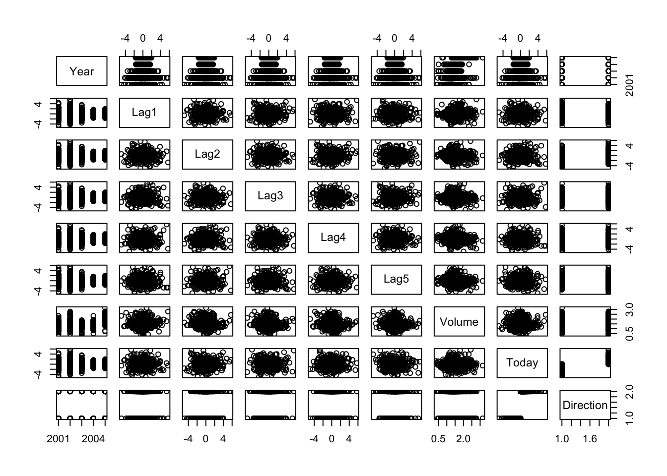
pairs(Smarket)
###

cor(Smarket[, -9])
###
attach(Smarket)
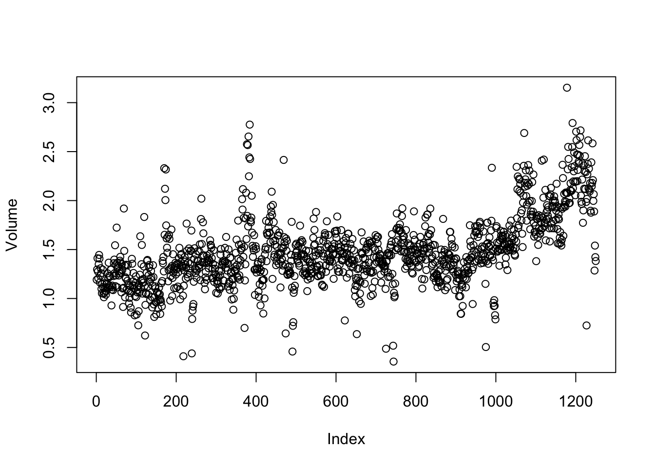
plot(Volume)

## Logistic Regression

###
glm.fits <- glm(
  Direction ~ Lag1 + Lag2 + Lag3 + Lag4 + Lag5 + Volume,
  data = Smarket, family = binomial
)
##family=binomial tells R to use logistic regression????mary(glm.fits)
###
coef(glm.fits)
summary(glm.fits)
# Null deviance: deviance for just mean(if you only use mean model it is log likelihood
#Residual deviance: deviance for the model with all the predictors in 
#(e.g. 1731,1249 df;1727,1243 df)
#? r上的glm对于binary就是logistic？
#? LDA的coefficient是怎么生成的（原理）（by hand e.g.)
summary(glm.fits)$coef
summary(glm.fits)$coef[, 4]
###
glm.probs <- predict(glm.fits, type = "response")#response variable, as opposite to omitting or type=link
glm.probs[1:10]
contrasts(Direction)
###

glm.pred <- rep("Down", 1250)
glm.pred[glm.probs > .5] = "Up"