ODE, PDE, and Fourier Series with codes
ODE, PDE, and Fourier Series
homogeneous ODE system in the two-compartment model
Laplace transform method for ODE system
characteristic equation method for ODE system
eigenvalue and eigenvector
numerical method for ODE system
# 加载所需的包
library(deSolve)

# 定义数值解函数
numeric_solution <- function(k01, k12, k21, k10, time) {
    # 定义ODE系统
    ode_system <- function(t, state, parameters) {
        A0 <- state["A0"]
        A1 <- state["A1"]
        A2 <- state["A2"]
        k01 <- parameters["k01"]
        k12 <- parameters["k12"]
        k21 <- parameters["k21"]
        k10 <- parameters["k10"]
        dA0_dt <- -k01 * A0
        dA1_dt <- k01 * A0 - (k12 + k10) * A1 + k21 * A2
        dA2_dt <- k12 * A1 - k21 * A2
        list(c(dA0_dt, dA1_dt, dA2_dt))
    }

    # 初始状态
    initial_state <- c(A0 = 1, A1 = 0, A2 = 0)
    parameters <- c(k01 = k01, k12 = k12, k21 = k21, k10 = k10)

    # 求解ODE
    solution <- ode(
        y = initial_state,
        times = time,
        func = ode_system,
        parms = parameters
    )

    # 转换为数据框
    solution_df <- as.data.frame(solution)
    out <- data.frame(
        time = solution_df$time,
        amount = solution_df$A1,
        solution = "numeric"
    )
    return(out)
}

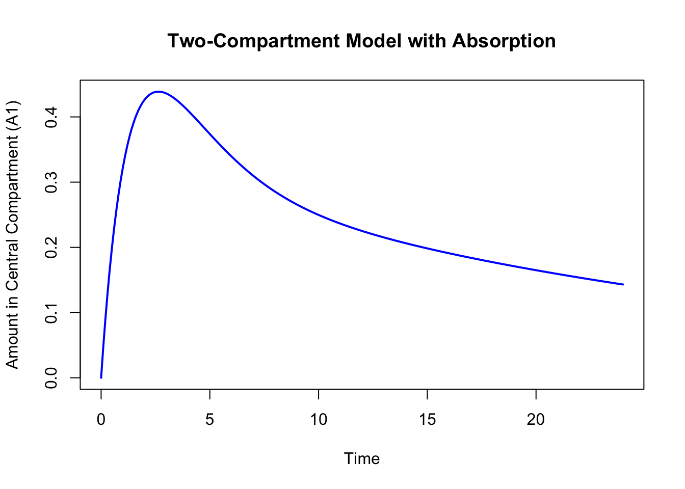
k01 <- 0.5  # 吸收速率常数
k12 <- 0.3  # 从中央室到周边室的分布速率常数
k21 <- 0.2  # 从周边室到中央室的分布速率常数
k10 <- 0.1  # 消除速率常数
time <- seq(0, 24, by = 0.1)  # 时间点从0到24小时

result <- numeric_solution(k01, k12, k21, k10, time)

head(result)

plot(result$time, result$amount, type = "l",
     xlab = "Time", ylab = "Amount in Central Compartment (A1)",
     main = "Two-Compartment Model with Absorption",
     col = "blue", lwd = 2)

# 加载所需的包
library(deSolve)
library(ggplot2)

# 定义数值解函数
numeric_solution <- function(k01, k12, k21, k10, time) {
    # 定义ODE系统
    ode_system <- function(t, state, parameters) {
        A0 <- state["A0"]
        A1 <- state["A1"]
        A2 <- state["A2"]
        k01 <- parameters["k01"]
        k12 <- parameters["k12"]
        k21 <- parameters["k21"]
        k10 <- parameters["k10"]
        dA0_dt <- -k01 * A0
        dA1_dt <- k01 * A0 - (k12 + k10) * A1 + k21 * A2
        dA2_dt <- k12 * A1 - k21 * A2
        list(c(dA0_dt, dA1_dt, dA2_dt))
    }

    # 初始状态
    initial_state <- c(A0 = 1, A1 = 0, A2 = 0)
    parameters <- c(k01 = k01, k12 = k12, k21 = k21, k10 = k10)

    # 求解ODE
    solution <- ode(
        y = initial_state,
        times = time,
        func = ode_system,
        parms = parameters
    )

    # 转换为数据框
    solution_df <- as.data.frame(solution)
    out <- data.frame(
        time = solution_df$time,
        amount = solution_df$A1,
        solution = "numeric"
    )
    return(out)
}

# 定义解析解函数
analytic_solution <- function(k01, k12, k21, k10, time) {
    ks <- k10 + k12 + k21
    alpha <- (ks + sqrt(ks^2 - (4 * k10 * k21))) / 2
    beta <- (ks - sqrt(ks^2 - (4 * k10 * k21))) / 2

    A <- (alpha - k21) / (alpha - beta)
    B <- -(beta - k21) / (alpha - beta)

    A_term <- A * exp(-alpha * time) * (exp(time * (alpha - k01)) - 1)
    B_term <- B * exp(-beta * time) * (exp(time * (beta - k01)) - 1)

    A_term <- A_term * k01 / (alpha - k01)
    B_term <- B_term * k01 / (beta - k01)

    out <- data.frame(
        time = time,
        amount = A_term + B_term,
        solution = "analytic"
    )
    return(out)
}

# 设置参数
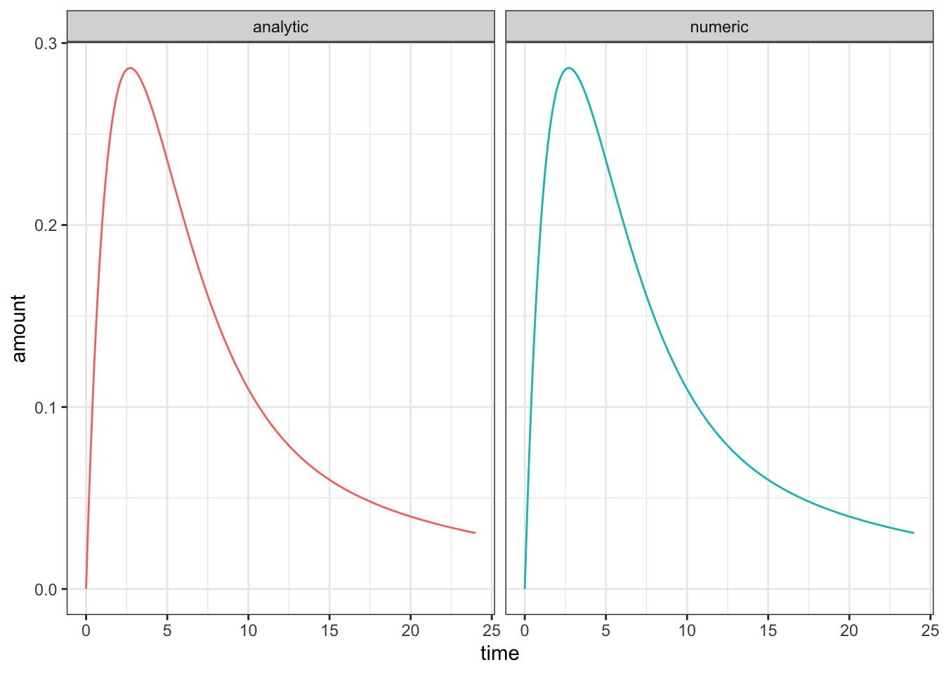
k01 <- 0.3
k12 <- 0.2
k21 <- 0.1
k10 <- 0.3
time <- seq(0, 24, 0.1)

# 计算数值解和解析解
dat_numb <- numeric_solution(k01, k12, k21, k10, time)
dat_anal <- analytic_solution(k01, k12, k21, k10, time)

# 合并数据
dat <- rbind(dat_numb, dat_anal)

# 绘制图形
ggplot(dat, aes(time, amount, colour = solution)) +
    geom_line(show.legend = FALSE) +
    facet_wrap(~solution) +
    theme_bw()
A difficult quesiton about variation parameters method for a 1st order ODEs
Find the solution of the equation
\[\frac{dy}{dx} - P(x)y = e^{2x}, \quad y(0) = 1,\]where \(P(x) = \begin{cases} 1 & x \in [0,1), \\ 0 & x \notin [0,1). \end{cases}\)
[Solution:] Consider the homogeneous equation
\[\frac{dy}{dx} - P(x)y = 0,\]| by separating the variables we have $\frac{dy}{y} = P(x)dx$, namely $\ln | y | = \int_0^x P(t)dt + C_1$, and we get |
Now by variation of parameters we suppose $u = u(x)$, and $y = u(x)e^{\int_0^x P(t)dt}$ is the solution, hence
\[u'(x) = e^{2x - \int_0^x P(t)dt} = \begin{cases} e^{2x} & x < 0, \\ e^x & x \in [0,1), \\ e^{2x-1} & x \geq 1. \end{cases}\](this is because :
The differential equation is given by: \(y' + p(x)y = f(x).\)
Integrating factor is: \(e^{\int p(x)dx}.\)
Multiplying through by the integrating factor: \(\frac{d}{dx} \left[ e^{\int p(x)dx} y \right] = f(x) e^{\int p(x)dx}.\)
Solving for $y$:
\[y e^{\int p(x)dx} = \int f(x) e^{\int p(x)dx} dx + C.\]Thus, the general solution is: \(y = Ce^{-\int p(x)dx} + e^{-\int p(x)dx} \int f(x) e^{\int p(x)dx} dx,\) where $y_c$ represents the complementary solution $Ce^{-\int p(x)dx}$ and $y_p$ represents the particular solution $e^{-\int p(x)dx} \int f(x) e^{\int p(x)dx}$.
)
and $C(0) = 1$ since $y(0) = 1$.
We see that
\[u(x) = u(0) + \int_0^x u'(t)dt = \begin{cases} \frac{e^{2x} + 1}{2} & x < 0 \\ e^x & x \in [0,1) \\ \frac{e^{2x-1} + e}{2} & x \geq 1. \end{cases}\]Finally we get
\[y = \begin{cases} \frac{e^{2x} + 1}{2} & x < 0 \\ e^{2x} & x \in [0,1) \\ \frac{e^{2x} + e^2}{2} & x \geq 1. \end{cases}\]Read “Differential Equations with Applications and Historical Notes” by George F. Simmons
Differential equations are the heart of analysis, which is the natural goal of elementary calculus and the most important part of mathematics for understanding the physical sciences.
Fourier Series
We can use functions in a orthogonal set,
\[\left\{ 1, \cos\left(\frac{\pi}{p}x\right), \cos\left(\frac{2\pi}{p}x\right), \cos\left(\frac{3\pi}{p}x\right), \ldots, \sin\left(\frac{\pi}{p}x\right), \sin\left(\frac{2\pi}{p}x\right), \sin\left(\frac{3\pi}{p}x\right), \ldots \right\}\](similar to a orthognal basis in linear algebra, to obtain the Fourier series). Specifically, we start with the orthogonal set {1, sin, cos, …}. By projecting the function onto these basis functions or computing the inner product three times—(f, 1), (f, cos), and (f, sin)—we can derive the Fourier series representation of the function.
Proof
Orthogonality isolates the constant Fourier coefficient by integrating against 1 over a full period.
Integrating against a cosine basis function isolates the corresponding cosine coefficient.
Integrating against a sine basis function isolates the corresponding sine coefficient.
THM
piecewise continuous function
- A function f(x) is piecewise continuous on an interval [a, b] if it is continuous on each subinterval (open interval) of [a, b] and has a finite number of (or jump) discontinuities in the interval. The function can be defined in pieces, and at each piece, it must be continuous.
thm–condition for convergence
f, and f’ are piecewise continuous on [-p,p], then for every x $\in $ [-p,p], the Fourier series of f(x) converges to f(x) at every point x in [-p,p] where f is continuous. If f has a jump discontinuity at x, the Fourier series converges to the average of the left-hand and right-hand limits of f at x.
Integrating factor is the translation of the diffrentiation operation
$y’+ky = f(x)$ is just $(D+k)y=f(x)$–> y=1/(D+k)f(x)
- idea : integrating factor and exact differential
$e^{kx} (y’+ky) =e^{kx} f(x)$
$ye^{kx} = \int e^{kx} f(x) dx$
y= $\frac{1}{e^{kx}} \int e^{kx} f(x) dx$ = $e^{-kx} \int^m e^{km} f(m) dm$–convolution
So the solution of y = $\frac{1}{e^{kx}} \int e^{kx} f(x) dx$ is the same as the solution of y=1/(D+k)f(x)
eg. $1/(D-2) (xe^x) = e^{-2x} \int e^{x} e^{2x} x dx = e^{-2x} \int e^{3x} x dx = e^{-2x} (e^{3x} (1/3)x - 1/9 e^{3x}) = 1/3 x e^x - 1/9 e^x$
result <- 0.927 /6


tan(5.356)

atan(5.356)

tan(-0.9271752)


0.8*cos(8 *pi/12)
0.8*cos(8 *pi/8)
0.8*cos(8 *pi/6)
0.8*cos(8 *pi/4)
0.8*cos(8 * (9*pi/32))

0.8*cos(8 * 3*pi/16)


-6.4*sin(8*3*pi/16)
use this idea we introduce the method of variation of parameters of finding the particular solution of the non-homogeneous linear equation system
….
method of using the matrix exponential to solve the system of ODEs
We can differentiate $e^{tA}$ with respect to $t$ and obtain
\(\begin{align*} \frac{d}{dt} e^{tA} &= A + tA^2 + \frac{t^2}{2!}A^3 + \frac{t^3}{3!}A^4 + \cdots \\ &= A \left( 1 + tA + \frac{t^2}{2!}A^2 + \frac{t^3}{3!}A^3 + \cdots \right) \\ &= Ae^{tA} \end{align*}\) as one would expect from differentiating the exponential function. We can therefore formally write the solution of
\[\dot{x} = Ax \qquad x(0) = e^{tA}x(0)\]If the matrix $A$ is diagonalizable such that $A = S\Lambda S^{-1}$, then observe that
\[\begin{align*} e^{tA} &= e^{tS\Lambda S^{-1}} \\ &= I + tS\Lambda S^{-1} + \frac{t^2(S\Lambda S^{-1})^2}{2!} + \frac{t^3(S\Lambda S^{-1})^3}{3!} + \cdots \\ &= I + tS\Lambda S^{-1} + \frac{t^2 S\Lambda^2 S^{-1}}{2!} + \frac{t^3 S\Lambda^3 S^{-1}}{3!} + \cdots \\ &= S \left( I + t\Lambda + \frac{t^2\Lambda^2}{2!} + \frac{t^3\Lambda^3}{3!} + \cdots \right) S^{-1} \\ &= Se^{t\Lambda}S^{-1} \end{align*}\]If $\Lambda$ is a diagonal matrix with diagonal entries $\lambda_1, \lambda_2,$ etc., then the matrix exponential $e^{t\Lambda}$ is also a diagonal matrix with diagonal entries given by $e^{\lambda_1 t}, e^{\lambda_2 t},$ etc.
We can now use the matrix exponential to solve a system of linear differential equations.
$\textbf{Example: Solve the previous example}$
\[\mathbf{X}' = \begin{pmatrix} 4 & 4 & 4 \\ 4 & 4 & 4 \\ -8 & -8 & -8 \end{pmatrix} \mathbf{X}\]We could use the traditional method of finding eigenvalues and eigenvectors, but more quicker is to use the matrix exponential since
\[A^2=\begin{pmatrix} 4 & 4 & 4 \\ 4 & 4 & 4 \\ -8 & -8 & -8 \end{pmatrix}\begin{pmatrix} 4 & 4 & 4 \\ 4 & 4 & 4 \\ -8 & -8 & -8 \end{pmatrix}=\begin{pmatrix} 0 & 0 & 0 \\ 0 & 0 & 0 \\ 0 & 0 & 0 \end{pmatrix}\]So we have $e^{At}=I+At$
Therefore, the solution of this system is $e^{At}\vec C =e^{At}(C_1,C_2,C_3)$, which is
\[X(t) = \begin{pmatrix} C_1 + 4t(C_1 + C_2 + C_3) \\ C_2 + 4t(C_1 + C_2 + C_3) \\ C_3 - 8t(C_1 + C_2 + C_3) \end{pmatrix}\]$\textbf{Example: Solve the previous example}$
\[\frac{d}{dt} \begin{pmatrix} x_1 \\ x_2 \end{pmatrix} = \begin{pmatrix} 1 & 1 \\ 4 & 1 \end{pmatrix} \begin{pmatrix} x_1 \\ x_2 \end{pmatrix}\]by matrix exponentiation.
We know that
\[\Lambda = \begin{pmatrix} 3 & 0 \\ 0 & -1 \end{pmatrix}, \quad S = \begin{pmatrix} 1 & 1 \\ 2 & -2 \end{pmatrix}, \quad S^{-1} = \frac{1}{4} \begin{pmatrix} -2 & -1 \\ -2 & 1 \end{pmatrix}.\]The solution to the system of differential equations is then given by
\[\begin{align*} x(t) &= e^{tA}x(0) \\ &= S^{A}S^{-1}x(0) \\ &= \frac{1}{4} \begin{pmatrix} 1 & 1 \\ 2 & -2 \end{pmatrix} \begin{pmatrix} e^{3t} & 0 \\ 0 & e^{-t} \end{pmatrix} \begin{pmatrix} -2 & -1 \\ -2 & 1 \end{pmatrix} \times (0). \end{align*}\]Successive matrix multiplication results in \(\begin{align*} x_1(t) &= \frac{1}{4}(2x_1(0) + x_2(0))e^{3t} + \frac{1}{4}(2x_1(0) - x_2(0))e^{-t}, \\ x_2(t) &= \frac{1}{2}(2x_1(0) + x_2(0))e^{3t} - \frac{1}{2}(2x_1(0) - x_2(0))e^{-t}. \end{align*}\)
Plz write the Cauchy-Euler equation as the simplest one and THEN use the method of variation of parameters!!!
Motivation from Professor Chi-Kun Lin: Differential equations reveal the secrets of nature even before we solve them. DEs are really related to the nature.
Eg of Variation of Parameters introduced by Professor Chi-Kun Lin:
The method of variation of parameters is a clever and elegant approach in solving non-homogeneous differential equations, especially in the context of physics. When we consider a differential equation, the non-homogeneous term F(x) can be seen as an external force acting on the system. In the absence of this force, the solution space of the homogeneous equation is spanned by a set of linearly independent solutions, such as $y_1$ and $y_2$. These solutions form the basis of the homogeneous solution through linear combinations.
However, when the external force $F(x)$ is introduced, it perturbs the system and necessitates the inclusion of a particular solution that specifically responds to this force. This particular solution still involves the original basis functions $y_1$ and $y_2$, but it introduces new coefficients $u_1(x)$ and $u_2(x)$ that are functions of the independent variable $x$. These coefficients are not constants; instead, they vary in a way that reflects the influence of the external force. The idea is that these coefficients $u_1(x)$ and $u_2(x)$ can be adjusted to account for the systematic changes induced by the physical quantity represented by $F(x)$.
The brilliance of the variation of parameters method lies in its ability to construct a particular solution by allowing these coefficients to vary. This method hypothesizes that by introducing these variable coefficients, the particular solution can effectively capture the response of the system to the external force. And indeed, this construction turns out to be effective. It provides a systematic way to find a particular solution that complements the homogeneous solution, thereby giving us the complete solution to the non-homogeneous differential equation. The name “variation of parameters” aptly describes the essence of this method, emphasizing the dynamic adjustment of the parameters (coefficients) in response to the external force.
Eg of the behind story of “Euler-Lagrange Equation”
$\frac{d}{dt}\frac{\partial L}{\partial q^{`}\alpha}-\frac{\partial L}{\partial q \alpha}$
While it’s often said that Lagrange was Euler’s student and that Euler had already discovered some of Lagrange’s work but chose not to publish to allow Lagrange to gain recognition, the reality of their relationship was a bit more nuanced.
Euler was indeed supportive of Lagrange’s work and recognized his talent. At the age of 19, Lagrange had made significant contributions to mathematics that caught Euler’s attention. Lagrange sent Euler his work on the calculus of variations, and Euler was very supportive. He recognized Lagrange’s talents and helped introduce him to the wider mathematical community.
Euler held back his own work on the calculus of variations to let Lagrange publish first. When Euler left Berlin for St. Petersburg in 1766, he recommended that Lagrange succeed him as the director of the Berlin Academy. This act was seen as a testament to Euler’s generous spirit and his recognition of Lagrange’s abilities.
Intro
To study ODEs and PDEs, the thinking way of Linear Algebra should be used!
$x^{(2)}$= x’’ = $\frac {d^2 x}{dy^2}$–this notation of the second order’s is actually share the same idea of “division”
Order
Liniarity
$a_n(x) \frac{d^n y}{dx^n } + … +a_1(x) \frac{d y}{dx } +a_0(x)y =g(x) $
- eg
(y-x)dx+4xdy=0
- $\frac {d^2 y}{dx^2}+\sin y=0$ is not linear since it has nonlinear function of y
solution of an ODE
? why continuous? —
An funtion defined on an interval I and possessing at least n derivatives that are continuous on I, which when substituted into an nth-order ordinary differential equation reduces the equation to an identity, is said to be a solution of the equation on the interval.
We cannot think solution of an ordinary differential equation without simultaneously thinking interval.
trivial solution –y=0, I
Solution Curve SEE CODEs
Explicit and implicit solution shape of ODEs
Singular solution
A solution of a system
System:
\(\cases{^{{\frac{dx}{dt}}=f(t,x,y)} _{\frac{dy}{dt}=g(t,x,y)}}\) Solution: x =$\Phi_1(t)$, y=$\Phi_2(t)$ defined on a common interval I that satisfy each equation of the system on this interval.
Initial Value Problem –codes
- def
On some interval I containing $x_0$, the problems of solving an nth-order DE subject to n side conditions (initial conditions (IC)) specified at $x_0$
An initial-value problem combines a differential equation with the values prescribed at the initial point.
Existence and Uniqueness
Does a solution of the problem exist? If a solution exists, is it unique?
Existence asks whether a solution curve passes through the initial value; uniqueness asks whether more than one can do so.
Interval of Existence and Uniqueness
Suppose y(x) represents a solution of the first order initial- value problem. The following three sets on the real x-axis may not be the same:
the domain of the function y(x), D
the interval I over which the solution y(x) is defined or exists,
and the interval $I_0$ of existence and uniqueness.
$I_0 \subseteq I \subseteq D$
Differential Equations as Mathematical Models
Newton’s law
Autonomous 1st Order DEs
for y(x): $\frac{dy}{dx} = f(y)$
Critical Points (equilibrium point/ stationary point)–f(y)=0
- eg. Population increase model
$\frac{dp}{dt} = p(a-bp)$
let f(p)=p(a-bp)=0 and catogorize the x-axis based on it, discussing the different situation intuitively
The phase line for the logistic equation marks the equilibria and the direction of change between them.
Properties of the solutions of autonomous DE
- A solution curve A solution curve follows the direction field determined by the autonomous equation.
? Translation Property–only autonomous DEs has this property?
- meaning: translation? A horizontal shift of an autonomous-equation solution is another solution because the equation has no explicit time dependence.
If y(x) is a solution of an autonomous differential equation dy ∕dx = f(y), then y1(x) = y(x − k) (y of (x-k)), k a constant, is also a solution.
Separable Equations
$\frac {dy}{dx}=g(x)h(y)$
singular solution
$\frac {dy}{h(y)}=g(x)dx$. If r is a zero of the function h(y), substituting y=r into dy/dx=g(x)h(y) makes both sides zero (y = r is a constant solution of the differential equation). As a consequence, y = r might not show up in the family of solutions that are obtained after integration and simplification. Such a solution is called a singular solution.
initial value problem
intergral-defined function
The integral form of a separable equation expresses the solution through accumulated change.
- eg
The worked separable-equation example applies the initial value after integration.
Linear equation
$a_1(x)\frac{dy}{dx}+a_0(x)y=g(x)$ is said to be a linear equation in the variable y.
- standard form:
$\frac{dy}{dx}+P(x)y=f(x)$
Integrating factor method
solution
idea: want to written into $\frac{d}{dx}()=f(x)$ then we assume after multiplying a factor $\mu(x)$ we can write $\frac{d}{dx}(\mu(x)y(x))=\mu(x)f(x)$
we get $\mu(x) = ce^{\int{p(x)dx}{}}$.
let c=1 we get the integrating factor
IVP
The integrating-factor solution uses the initial condition to determine its integration constant.
?Error function
The diagram tracks the error between an exact solution and its approximation.
The companion diagram compares the approximation with the solution over the interval.
Exact equations
z=f(x,y)=c
Non-exact
Bernouli’s equation
DO Not Remember–understand it instead!
just want to transform the equation to a 1st order differential equation to solve it using integrating factor method.
W7
Homogeneous Linear System
Just follow the idea in $y’‘+my’+ny=0$, when facing the linear system $\cases{{\vec {x’} = A\vec x}\{ay’+by=0}}$, we also assume that $\vec {x’} = \vec ke^{\lambda t}$ and substitute it into $\vec {x’} = Ax$
phase portrait and stable/ unstable / semi-stable points
? JORDAN FORM AND ODE system?
When we solve $ay’‘+by’+cy=0$ if m is a double root, then $y_1=e^{mx}$, $y_2=xe^{mx}$
Naturally, here we assume $\vec x_2 =\vec k t e^{\lambda t}$, substitute $\vec x_2$ into the system $\vec {x’} = Ax$;
LHS = $\vec {x_2’} = \vec k(e^{\lambda t }+\lambda te^{\lambda t})=A\vec x_2$=$A\vec k t e^{\lambda t}$ =RHS
Then we get $\vec k = \vec 0$.
So our assumption is not true.
There is an extra term
对称矩阵重复n次的eigenvalue一定能找到n个线性无关的特征向量
把一个矩阵化为对角矩阵 (gauss- Jordan elimination)
##
ODEs and PDEs with codes
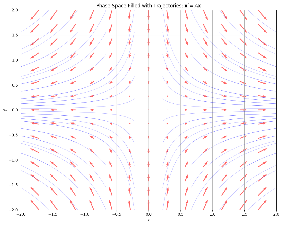
To solve the linear ODE $ \mathbf{x}’ = A\mathbf{x} $ and visualize how different initial conditions affect the trajectories, we can use a saddle point matrix $ A $ with eigenvalues of opposite signs. This setup results in varied trajectory shapes such as diverging, converging, and hyperbolic paths depending on the initial conditions.
Explanation:
- Matrix $ A $: The chosen matrix $ A = \begin{bmatrix} 1 & 0 \ 0 & -1 \end{bmatrix} $ has eigenvalues $ 1 $ and $ -1 $, creating a saddle point. This results in:
- Unstable manifold (x-axis): Initial conditions along the x-axis diverge exponentially.
- Stable manifold (y-axis): Initial conditions along the y-axis converge to the origin.
- Hyperbolic trajectories: Other initial conditions follow hyperbolic paths, curving away in x and converging in y (or vice versa).
-
Integration: The ODE is solved numerically using
solve_ivpfor each initial condition, generating trajectories over the time span $ t \in [0, 3] $. - Visualization: Trajectories are plotted in the phase plane, demonstrating how different initial values lead to distinct curve shapes (diverging lines, converging lines, hyperbolas).
By adjusting the initial conditions, you can observe how trajectories evolve according to the eigenvectors and eigenvalues of $ A $, illustrating the system’s dynamic behavior.
import numpy as np
from scipy.integrate import solve_ivp
import matplotlib.pyplot as plt

# Define the matrix A (saddle point)
A = np.array([[1, 0],
              [0, -1]])

def ode_system(t, x):
    return A @ x

# Time span for integration
t_span = (0, 3)
t_eval = np.linspace(t_span[0], t_span[1], 100)

# Generate a grid of initial conditions
x_vals = np.linspace(-2, 2, 10)  # 20 points from -2 to 2 in x
y_vals = np.linspace(-2, 2, 10)  # 20 points from -2 to 2 in y
X, Y = np.meshgrid(x_vals, y_vals)
initial_conditions = np.vstack([X.ravel(), Y.ravel()]).T  # 400 initial points

# Plot settings
plt.figure(figsize=(10, 8))
plt.title('Phase Space Filled with Trajectories: $\mathbf{x}\' = A\mathbf{x}$')
plt.xlabel('x')
plt.ylabel('y')

# Plot trajectories for all initial conditions
for x0 in initial_conditions:
    sol = solve_ivp(ode_system, t_span, x0, t_eval=t_eval)
    plt.plot(sol.y[0], sol.y[1], color='blue', alpha=0.4, linewidth=0.5)

# Overlay the vector field for context
x_grid, y_grid = np.meshgrid(np.linspace(-2, 2, 15), np.linspace(-2, 2, 15))
dxdt = A[0, 0] * x_grid + A[0, 1] * y_grid
dydt = A[1, 0] * x_grid + A[1, 1] * y_grid
plt.quiver(x_grid, y_grid, dxdt, dydt, color='red', alpha=0.6,
           scale=50, width=0.003, headwidth=3)

plt.grid(True)
plt.xlim(-2, 2)
plt.ylim(-2, 2)
plt.tight_layout()
plt.show()
Key Modifications:
- Grid of Initial Conditions:
- A 8x8 grid of initial points is generated using
np.meshgrid, covering the region $[-2, 2] \times [-2, 2]$. - This creates 64 trajectories, densely filling the phase space.
- A 8x8 grid of initial points is generated using
- Trajectory Styling:
- Trajectories are plotted with low
alpha(transparency) and thin lines to avoid visual clutter. - All trajectories use the same color (
blue) to emphasize collective behavior.
- Trajectories are plotted with low
- Vector Field Overlay:
- A quiver plot (red arrows) is added to show the direction of the vector field $ \mathbf{x}’ = A\mathbf{x} $, providing context for the trajectories.
Result:
- The plot will show:
- Diverging paths along the unstable manifold (x-axis).
- Converging paths along the stable manifold (y-axis).
- Hyperbolic curves elsewhere, filling the phase space.
- The saddle-point dynamics are clearly visible, with trajectories stretching outward in $x$ and contracting in $y$.
Adjustments for Speed/Resolution:
- Reduce the grid resolution (e.g.,
np.linspace(-2, 2, 10)for 10 points) for faster execution. - Increase
alphaorlinewidthto make trajectories more prominent.
To visualize the phase space filled with trajectories, we can generate a grid of initial conditions and plot their paths. Here’s a modified version of the code that densely fills the phase portrait:
import numpy as np
from scipy.integrate import solve_ivp
import matplotlib.pyplot as plt

# Define Lotka-Volterra parameters (α=prey growth, β=predation, δ=predator growth, γ=predator death)
α, β, γ, δ = 1.5, 0.5, 0.5, 0.5

def lotkavolterra(t, z):
    x, y = z
    dxdt = α * x - β * x * y
    dydt = δ * x * y - γ * y
    return [dxdt, dydt]

# Time span and grid setup
t_span = (0, 15)
t_eval = np.linspace(t_span[0], t_span[1], 500)

# Generate a grid of initial conditions (avoid x=0 or y=0 to skip trivial solutions)
x0_vals = np.linspace(0.5, 5, 8)  # Prey population
y0_vals = np.linspace(0.5, 5, 8)  # Predator population
X0, Y0 = np.meshgrid(x0_vals, y0_vals)
initial_conditions = np.vstack([X0.ravel(), Y0.ravel()]).T

# Plot setup
plt.figure(figsize=(10, 8))
plt.title("Lotka-Volterra Phase Portrait: Predator-Prey Dynamics")
plt.xlabel("Prey Population ($x$)")
plt.ylabel("Predator Population ($y$)")

# Solve and plot trajectories for all initial conditions
for x0, y0 in initial_conditions:
    sol = solve_ivp(lotkavolterra, t_span, [x0, y0], t_eval=t_eval)
    plt.plot(sol.y[0], sol.y[1], color='blue', alpha=0.3, linewidth=0.7)

# Overlay the vector field (quiver plot)
x_grid, y_grid = np.meshgrid(np.linspace(0, 5, 20), np.linspace(0, 5, 20))
dx, dy = np.zeros_like(x_grid), np.zeros_like(y_grid)
for i in range(x_grid.shape[0]):
    for j in range(x_grid.shape[1]):
        dz = lotkavolterra(0, [x_grid[i,j], y_grid[i,j]])
        dx[i,j], dy[i,j] = dz[0], dz[1]
plt.quiver(x_grid, y_grid, dx, dy, color='red', alpha=0.6, scale=100, width=0.004)

# Mark the non-trivial fixed point (critical point)
fixed_point_x = γ / δ
fixed_point_y = α / β
plt.scatter(fixed_point_x, fixed_point_y, color='black', s=80, label=f'Fixed Point ({fixed_point_x:.1f}, {fixed_point_y:.1f})')

plt.xlim(0, 5)
plt.ylim(0, 5)
plt.legend()
plt.grid(True)
plt.tight_layout()
plt.show()
Key Features:
- Lotka-Volterra Dynamics:
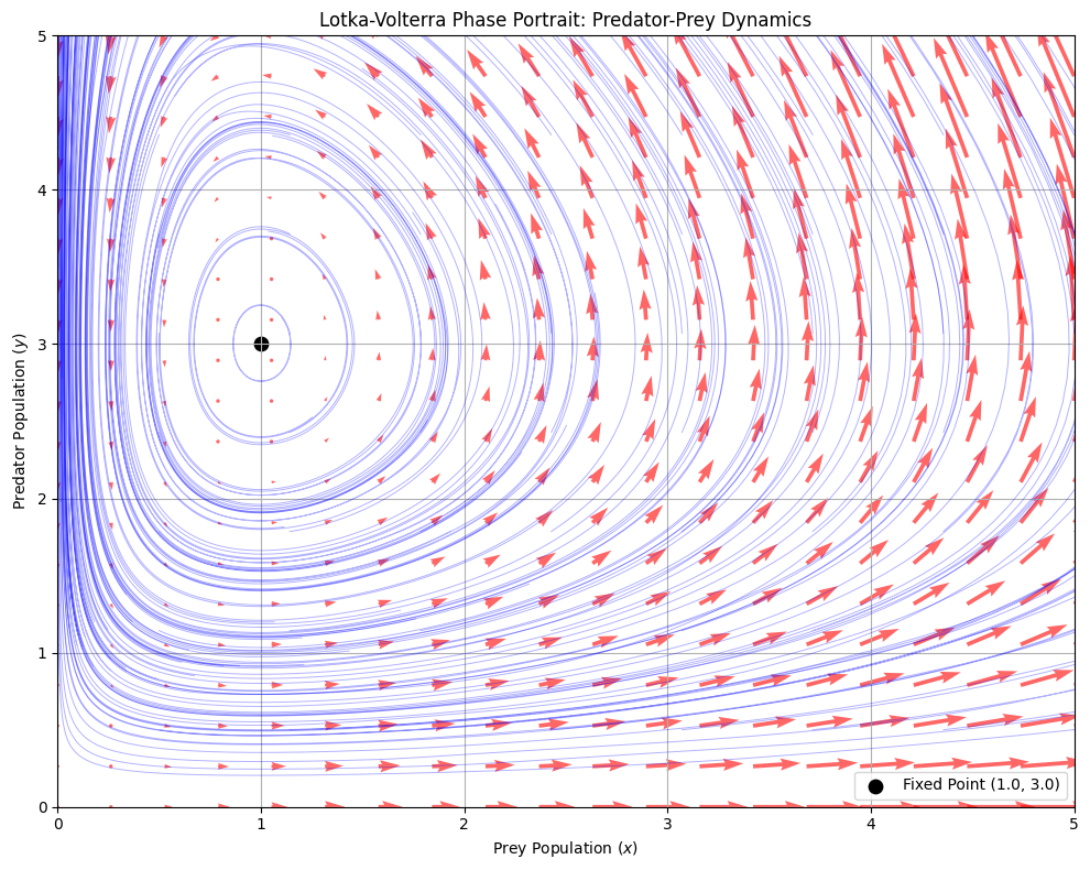
- Closed Orbits: Trajectories form periodic cycles (predator-prey oscillations).
- Fixed Point: The non-trivial equilibrium at $ (x^, y^) = (\gamma/\delta, \alpha/\beta) $, marked as a black dot.
- Grid of Initial Conditions:
- A 15×15 grid covers initial prey and predator populations in $ [0.5, 5] \times [0.5, 5] $.
- Avoids $ x=0 $ or $ y=0 $ (trivial equilibria where one species is extinct).
- Visual Enhancements:
- Trajectories: Plotted with transparency to show density of paths.
- Vector Field: Red arrows indicate the direction of the dynamics.
- Fixed Point: Highlights the center of the periodic orbits.
Result:
- The plot shows concentric cycles around the fixed point, illustrating how different initial populations lead to oscillations of varying amplitudes.
- All trajectories conserve a quantity (the “Hamiltonian” of the system), forming closed loops.
Adjustments to Explore:
- Change parameters $ \alpha, \beta, \gamma, \delta $ to shift the fixed point or alter oscillation frequencies.
- Extend the grid to larger populations (e.g.,
np.linspace(0.5, 10, 20)).
Yes! The classical Lotka-Volterra system (with parameters $ \alpha, \beta, \gamma, \delta $) has neutrally stable closed orbits (trajectories neither converge to nor diverge from the fixed point). However, if we modify the system to include damping (e.g., logistic growth for prey or predator saturation), the dynamics change: trajectories can spiral inward or outward depending on parameters. Below is an example of such a modified system where solutions converge to the fixed point.
Modified Lotka-Volterra System with Logistic Prey Growth
We add a logistic term $ \left(1 - \frac{x}{K}\right) $ to the prey equation, introducing a carrying capacity $ K $. This creates damped oscillations converging to the fixed point:
$ \begin{cases} \frac{dx}{dt} = \alpha x \left(1 - \frac{x}{K}\right) - \beta xy,
\frac{dy}{dt} = \delta xy - \gamma y. \end{cases} $
Parameter Setup for Convergence:
α = 1.0   # Prey growth rate
β = 0.2   # Predation rate
δ = 0.1   # Predator growth efficiency
γ = 0.5   # Predator death rate
K = 50    # Carrying capacity for prey (new parameter causing damping)
import numpy as np
from scipy.integrate import solve_ivp
import matplotlib.pyplot as plt

# Modified Lotka-Volterra with logistic prey growth
def modified_lotkavolterra(t, z, α, β, γ, δ, K):
    x, y = z
    dxdt = α * x * (1 - x/K) - β * x * y
    dydt = δ * x * y - γ * y
    return [dxdt, dydt]

# Parameters for damped oscillations
params = (1.0, 0.2, 0.5, 0.1, 50)  # α, β, γ, δ, K

# Time span and initial conditions
t_span = (0, 100)
t_eval = np.linspace(t_span[0], t_span[1], 1000)

# Initial conditions near the fixed point
initial_conditions = [
    [10, 5],
    [30, 15],
    [40, 25],
    [5, 20]
]

# Plot setup
plt.figure(figsize=(12, 6))

# Phase portrait
plt.subplot(1, 2, 1)
plt.title("Phase Portrait: Damped Oscillations")
plt.xlabel("Prey ($x$)")
plt.ylabel("Predator ($y$)")

# Time series
plt.subplot(1, 2, 2)
plt.title("Time Series: Prey and Predator")
plt.xlabel("Time")
plt.ylabel("Population")

# Solve and plot trajectories
for x0, y0 in initial_conditions:
    sol = solve_ivp(modified_lotkavolterra, t_span, [x0, y0], args=params, t_eval=t_eval)

    # Phase portrait
    plt.subplot(1, 2, 1)
    plt.plot(sol.y[0], sol.y[1], alpha=0.7, linewidth=1,
             label=f'IV: ({x0}, {y0})')

    # Time series
    plt.subplot(1, 2, 2)
    plt.plot(sol.t, sol.y[0], linestyle='--', alpha=0.7, linewidth=1)
    plt.plot(sol.t, sol.y[1], linestyle='-', alpha=0.7, linewidth=1)

# Overlay fixed point (phase portrait)
x_star = (γ / δ)  # Fixed point x-coordinate
y_star = (α / β) * (1 - x_star / params[-1])  # Fixed point y-coordinate (modified)
plt.subplot(1, 2, 1)
plt.scatter(x_star, y_star, color='red', s=100, zorder=10, label='Stable Fixed Point')
plt.legend()
plt.grid(True)
plt.xlim(0, 60)
plt.ylim(0, 30)

# Finalize plot
plt.tight_layout()
plt.show()
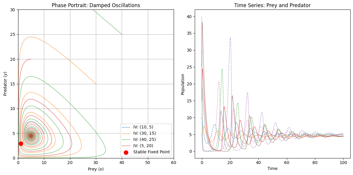
Key Results:
- Damped Oscillations:
- Trajectories spiral inward toward the fixed point $ (x^, y^) \approx (5.0, 4.75) $, demonstrating asymptotic stability (unlike classical Lotka-Volterra).
- Oscillation amplitudes decay over time due to the logistic term $ \left(1 - \frac{x}{K}\right) $.
- Fixed Point Stability:
- The Jacobian matrix at $ (x^, y^) $ has eigenvalues with negative real parts, causing convergence.
- The logistic term acts as a damping force, stabilizing the system.
Why This Works:
- Logistic Term: The term $ \left(1 - \frac{x}{K}\right) $ limits prey growth at high populations, breaking the conservation law of the classical model.
- Parameter Tuning: With $ K = 50 $, the damping effect is strong enough to suppress perpetual oscillations.
Adjustments:
- To see divergence (unstable fixed point), set $ K < \gamma/\delta $. Trajectories will spiral outward.
- Remove the logistic term ($ K \to \infty $) to recover classical neutrally stable orbits.
This modification shows how structural changes to the model (not just parameter tweaks) can dramatically alter stability.\
“A Kun’s PDE Lecture”
Fritz Jhon’s textbook
fibonacci sequence
菠萝和叶子
西方的智慧
Russel
分析的算术化
$f’(x)=lim_{x->x_0}f(x)-f(x_0)/x-x_0$
西方哲学史
球的表面积
微积分解决球的表面积
看课本
为什么这些概念不从小学引进
分析
-
function
-
continulity
-
differentiability
-
integralbility
what is a number
- Q, rational number q/p (ratio)
有理数用直尺画,根号用圆规–算术平均大于几何平均
什么是理性
古巴比伦用宗教解释不理解的事情
古希腊人(大自然是可理解的)带给现代人最珍贵的礼物就是理性
爱因斯坦:大自然最不可理解的地方是大自然竟然是可理解的
古希腊的传人
理性的工具是数学,希腊人对数学的重视
科技(建筑)和科学(要有主张和实验)
$\mathbb R$
E.Steim
分离变数法–傅立叶级数—分析
微积分
-
傅立叶 analysis
-
complex analysis
-
real analysis
-
functional analysis
convergence
- 有上界
- 有下界
- 柯西sequence
用多项式看函数
- Weierstrass Approximation Theorem(density)
所有函数在有界的闭区间都可以用多项式逼近
函数(function)()
math
geometry
the most important thing in geometry is about measure.
algebra
simplize authority独断权威
analysis
democracy
Newton
anatomy
f(x)约等于 $\Sigma a_nx^n$—-Talor series
be patient to learn analysis
Equations are expressing secrets in the nature!
We should feel them.
A healthy view of mathematics.
- We should have a healthy view of mathematics, including retrospect the whole process of math history which help us think a question as giants. The accumulation of many unsung heroes deserves our respect forever. We could not wait for a super giant, we should learn to think similarly as a super ancient giant. We should have the feeling of finding truth.—-Dr. Andrew Chi-kun Lin
History
Reformation
Renaissance
Enlightenment
Industrial Revolution
No dynasty lasts over 300 years, except Song dynasty which lasted over 300 years, with scholars serving as prime ministers. Su Shi snored.
Partial Differential Equations (PDE)
Complex functions are continuously differentiable and infinitely differentiable. 复变函数是连续可微,无穷多次可微
Differentiation at a point straight line, parabola (implying second-order differentiability). 在一点微分 直线 抛物线(隐含二次可微)
PDEs are harmonic functions; differentiating twice gives continuous results. pde是调和函数 微分两次是连续
Bootstrap.
Infinitely differentiable.
Intrinsic structure within itself.
Related to complex functions.
ODEs have only one variable.
Newton’s second law is an ODE (second-order ordinary differential equation), and then comes calculus.
After Newton, no one else appeared in Britain except Taylor—isolated, and Newton had terrible notation.
But Leibniz had the Bernoulli brothers—passion is everything.
“There is no royal road to geometry.”
Understand differentiation, grasp its essence, and find a way to integrate it back.
C1, C2: 2 constants are obtained by integrating twice.
\[z = u(x,y) \quad \text{2-dimensional}\] \[surface: z = f(x,y)\]Multivariable calculus focuses on understanding the surface and finding tangent planes, normal vectors, etc.
\[au_{xx} + bu_{xy} + cu_{yy} = f(u)\]Wave Equation
Vibration of a string.
Taylor, d’Alembert, Daniel Bernoulli, Jacob Bernoulli (Euler), Jacob Bernoulli (distribution).
\[\frac{d^2x}{dt^2}\]The truths of this world have all been discovered by Newton.
\[u(x,t) \text{: amplitude, } [u] = L\]$$ [p] = M/L
$$
\[p(x,t) \text{: density (1-dimensional)}\][T] = [ma] = [m][a] = ML/t\^2
$T=T_1=T_2$ tension
(0-L)
F = Tsin() - Tsin
m = $\rho$ x
2nd law: $\rho$ x
linear transformation
Keep the parallelogram diagonal 保持平行四边形的对角线 x+y
keep a straight line 保持直线—a
向量空间 vector space
如果是从二维映射到三维怎么办。2dim—3dim?
代数结构
保留加法 keep the addition
homomorphism
morphism–形象
1st Partial differential equation in the world
Found by Newton, solved by Dala, which is a spring. wave on a spring.
Based on force analysis, we know:
\(\rho \Delta x \frac{\partial^2 u}{\partial t^2} = T \sin(\theta + \Delta \theta) - T \sin(\theta)\) where $\Delta \theta$ is very small, so $sin\theta$=$tan\theta$
\[=T \frac{\partial u}{\partial x}\left( x + \Delta x, t \right) - T \frac{\partial u}{\partial x} (x, t)\]think of diffrential
\(T \frac{\partial^2 u}{\partial x^2}(x + \lambda \Delta x, t)\Delta x\) 想到微分– think of differential
\[\frac{\partial^2 u}{\partial x^2} = \frac{T}{\rho} \frac{\partial^2 u}{\partial t^2}\]The speed of the wave is:
\[C^2 = \frac{T}{\rho}\]Differential Equation: $u_{tt}-c^2u_{xx}=0, x\in[0,L]$
Boundary Condition: $u(0,t)=u(L,t)=0, t\geq 0$
Initial Condition: u(x,0)=f(x), $u_t(x,0)=g(x)$. —Newton 2nd law decides track
Da.. Bernulli Separation of Variables
$u(x,\theta)=\phi(x)T(t)$. (Gassian integral formula derivation also use this method)
(A continuous function can be approximated by a polynomial, which is a super polynomial)
(the defination of “density”)
(Seperation variable: God to God, Caesar to Caesar—-x to x, t to t)
分离变数
\[\frac{T^{''}(t)}{C^2 T(t)} = -\frac{\phi^{''}(x)}{\phi(x)}\] \[\begin{aligned} &\text{PDE:} \quad \text{分离变量法,separete variables} \rightarrow \text{ODE} \\ &\phi'' + \lambda \phi = 0 \\ &T'' + \lambda c^2 T = 0 \\ &\text{(B.C.) 边界条件:} \\ &u(0,t) = \phi(0) T(t) = 0 \quad \Rightarrow \quad \phi(0) = 0 \quad \text{(trivial 非平凡解,boring)} \\ &u(L,t) = \phi(L) T(t) = 0 \quad \Rightarrow \quad \phi(L) = 0 \end{aligned}\] \[\lambda < 0 \quad , \quad \phi = e^{mx} \quad \text{(不可能,从0到0。0--0, impossible)}\] \[\lambda = 0 \quad , \quad \phi = Ax + B \quad \text{直线运动, straight move}\]\(\lambda > 0 \quad , \quad \phi = c_1 \cos(\sqrt{\lambda} x) + c_2 \sin(\sqrt{\lambda} x)\) ### 解的推导
考虑方程: \(\phi'' + \lambda \phi = 0\) 其中 (\lambda) 是一个常数,解的形式取决于 (\lambda) 的值。
1. 当 (\lambda < 0)
当 (\lambda < 0) 时,我们令 (\lambda = -\mu\^2) ,于是方程变为: \(\phi'' - \mu^2 \phi = 0\) 其通解为: \(\phi(x) = A e^{\mu x} + B e^{-\mu x}\) 这种解形式表示指数发散或衰减,通常是不稳定解。
2. 当 (\lambda = 0)
当 (\lambda = 0) 时,方程变为: \(\phi'' = 0\) 这是一个线性方程,其通解为: \(\phi(x) = A x + B\) 这表示直线运动。
3. 当 (\lambda > 0)
当 (\lambda > 0) 时,我们令 (\lambda = \mu\^2) ,方程变为: \(\phi'' + \mu^2 \phi = 0\) 其解为: \(\phi(x) = A \cos(\mu x) + B \sin(\mu x) ---wave\) 这种解表示周期性波动。
推导
对于形如 ( $\phi’’ + \mu^2 \phi = 0$ ) 的常微分方程,我们可以猜测它的解是指数形式,即:
\[\phi(x) = e^{rx}\]这里 ( r ) 是需要确定的参数。
代入微分方程:
将 ( \phi(x) = e\^{rx} ) 代入原方程,得到:
\[r^2 e^{rx} + \mu^2 e^{rx} = 0\]由于 ( e\^{rx} \neq 0 ),可以消掉这个项,剩下的是特征方程:
\(r^2 + \mu^2 = 0\) 这个特征方程的解为:
\[r = \pm i \mu\]这是一个虚数解。
当特征根为纯虚数时,方程的通解可以写成正弦和余弦的组合形式,根据欧拉公式 ( e\^{i\mu x} = \cos(\mu x) + i \sin(\mu x) ),我们得到通解为:
\[\phi(x) = A \cos(\mu x) + B \sin(\mu x)\]其中,( A ) 和 ( B ) 是待定常数,它们可以通过边界条件或初始条件来确定。
characteristic
\[\phi(x) = C_1 \cos(\sqrt{\lambda}x) + C_2 \sin(\sqrt{\lambda}x)\]边界条件: \(\phi(0) = 0 \Rightarrow C_1 = 0\)
\[\phi(L) = C_2 \sin(\sqrt{\lambda}L) = 0\]因此, \(\sqrt{\lambda_n}L = n\pi \quad (n = 1, 2, 3, \dots)\)
得到本征值: \(\lambda_n = \left( \frac{n\pi}{L} \right)^2, \quad n = 1, 2, 3, \dots\)
对应的本征函数为: \(\phi_n(x) = \sin \left( \frac{n\pi x}{L} \right)\) Sturm-Liouville Problem:
\[\lambda_n = \left( \frac{n\pi}{L} \right)^2, \quad n = 1, 2, 3, \dots\]因此,特征函数为: \(\phi_n(x) = \sin \left( \frac{n\pi x}{L} \right)\) \(T_n(t) = C_1 \cos \left( \frac{n\pi c t}{L} \right) + C_2 \sin \left( \frac{n\pi c t}{L} \right)\)
\[u_n(x,t) = T_n(t) \phi_n(x)\]代入展开: \(u(x,t) = \sum_{n=1}^{\infty} C_n \sin \left( \frac{n\pi x}{L} \right) \left[ C_1 \cos \left( \frac{n\pi c t}{L} \right) + C_2 \sin \left( \frac{n\pi c t}{L} \right) \right]\)
Dimension
from Fourier
Dimensions help us to check the calculation, trigonometric functions have no dimensions, integrals do not change the overall dimension.
? 107
Only real number could be expressed as big or small, which is the only comperate order field 2-dim has norm
others
law of large number
eg. The reason the casino makes money is because even though the people who go there have a little more than a half chance of winning, the casino has more money than you, and if you stay long enough, you will win, so don’t go to the casino, because you can’t go deeper than the casino
analysis inequality
analysis is limit, limit is approximation, ## continuous proof of 2 continuous functions
f is continuous at $x_0$
is equal to
| For every $\varepsilon > 0$, there exists $\delta > 0$ such that if $ | x - x_0 | < \delta_1$, then $ | f(x) - f(x_0) | < \varepsilon$. |
g(x), also , delta_2
| $ | (f(x)+g(x))-(f(x_0)+g(x_0) | $ |
| =$ | (f(x)-f(x_0))+(g(x)-g(x_0) | $ |
triangle inequality
| =$\leq | f(x)-f(x_0) | + | g(x)-g(x_0) | $ |
= $1/2\varepsilon$+$1/2\varepsilon$
$\forall\varepsilon$ greater than 0, $\exists \delta=min({\varepsilon_1,\varepsilon_2})$
Does math have elements?
             ---Paul Halmos
             Geometric Series
1-ab and 1-ba —- invertible
I-AB invertible
— I-BA invertible (hint: $I+B(I-AB)^{-1}A$)
do not 杀鸡用牛刀—-
prove the harmonic series is divergent:
idea: geometric series:
1+1/2+(1/3+1/4)+….
1+(1/2+1/3)+(1/4+..+1/9)+(1/10+…+1/27)+…$\geq$ 1+(1/3)
which is relevant to fuliyejishu
学数学不要兵来将挡水来土掩,要有一个整套的思想,不要背书 idea: geometric series
(1-ba)^{-1}=1/1-ba=1+ba+baba+..=1+b(1+ab+abab+..)a=1+b(1-ab)^{-1}a
(1-ba)[1+b(1-ab)\^{-1}a]
1+b(1-ab)^{-1}a-ba-bab(1-ab)^{-1}a=(commutive law)=1-ba+b(1-ab)^{-1}a-bab(1-ab)^{-1}a=1-ba+b(1-ab)(1-ab)\^{-1}a
=1-ba+b1a
=1-ba+ba
=1 —-so do not recite boring things, remember based on understanding.
Do not read Gassian, read Oral
firstly, for matrix, AB $\noequal$ BA—-f(g) is not equal to g(f)
学学问要有感觉
chat with different famous … 西方的没落–fu springer
liangzilixue hysenber—max born
the true meaning of matrix is the linear transformation(fun f)
p-series
Integral test with dimensional analysis to know p>1 for convergence
$\sum_{n=1}^{\infty} \frac{1}{n^p} \approx \int_1^\infty 1/x^p \, dx\approx 1/[x]^p*[x]=[x]^{1-p} ([x]–>\infty)—>1-p\leq 0$
again, geometric series,
1/1^2+(1/2^2+1/3^2)+(1/4^2+..)
$\leq 1+(1/2^2+1/2^2)+$
= 1+2/2\^2 +4/4^2+8/8^2z=…=2
Euler
Euler idea: Viete fumula
relation of root and coefficient
$\sum_{n=1}^{\infty} \frac{1}{n^p}=\pi^2/6$
(x-a)(x-b)=x\^2-(a+b)x+ab
(1-x/a)(1-x/b)=1-(1/a+1/b)x+1/ab*x\^2
(1-x)(1+x)
(1-x)(1+x)(1-x/2)(1+x/2)
(1-x)(1+x)(1-x/2)(1+x/2)…(1-x/n)(1+x/n)+…
=1-(1/1^2+1/2^2+…+1/n^2)x^2+…
Q: find a function whose roots are +-1, +-2, +-3,….
so Euler changed this Q:
rewrite:
(1-x/\pi)(1+x/\pi)(1-x/2\pi)(1+x/2\pi)…
= 1-(1/1^2+1/2^2+1/n^2+…)1/^\pi2x\^2+…
先猜答案
guess sinx = (1-x/\pi)(1+x/\pi)…(1-x/n\pi)(1+x/n\pi)
but 0 is a solution
so change to sinx/x
sinx/x =k…..
k=limsinx/x=1
1/x is 振幅
sinx/x=1-(1/1^2+1/2^2+…+1/n^2+…)x^2/\pi\^2+…
=1/x
天才是创意
create a thery of math
and six/x = 1/x(x-x^3/3!+…)=1-x^3/6
so we know
Reference
林琦焜 (2001),從 Cantor 集到碎形。數學傳播,25(1),-。